Method 1 – Applying the RANDBETWEEN Function to Generate Random Data in Excel
Step 1:
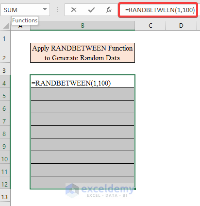
- Select the Cells to enter the random data. Here, B4:B12.
- Enter the formula.
=RANDBETWEEN(1,100)
The RANDBETWEEN function returns a random integer number between the specific numbers.
- Press CTRL+Enter.
Random integer numbers between 1 to 100 are displayed.
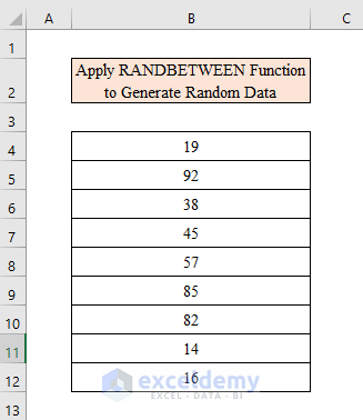
Duplicate values may appear.
Step 2:
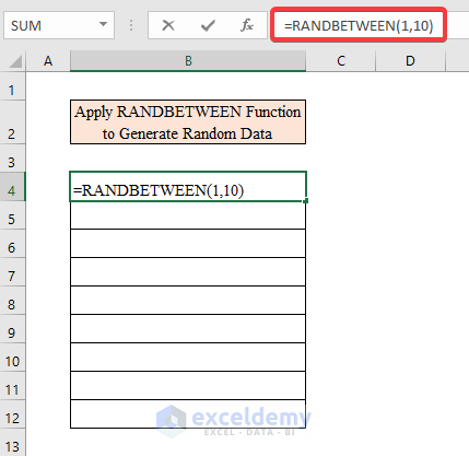
- Select the Cells to enter the random data.
- Enter the formula.
=RANDBETWEEN(1,10)
The RANDBETWEEN function returns integers between the given numbers.
- Press CTRL+Enter.
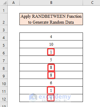
Duplicate values may appear.
Method 2 – Using the RAND Function to Generate Random Data in Excel
2.1 Generate Data Between 0 and 1
Steps:
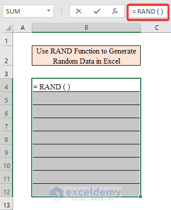
- Select the Cells to enter the random data.
- Enter the formula.
=RAND()
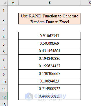
The RAND function will return a random number between 0 and 1.
- Press CTRL+Enter.
This is the output.
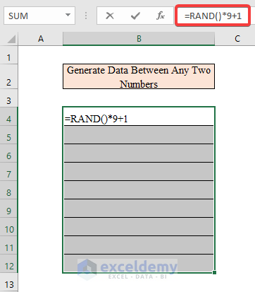
2.2 Generate Data Between Any Two Numbers
Steps:
- Select cells.
- Use the formula.
=RAND()*9+1
The RAND function returns random numbers within the given range.
- Press CTRL+Enter.
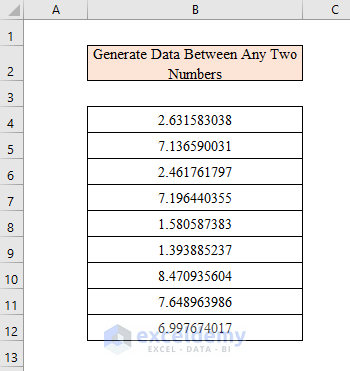
- Random decimal data between 1 and 10 will be displayed.
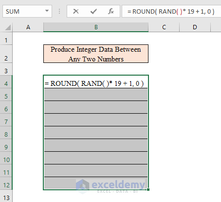
2.3 Generate Integer Data Between Any Two Numbers
Step 1:
- Select B4:B13.
- Enter the formula
= ROUND( RAND( ) * ( 19 +1 ), 0 )
The RAND function returns a random number within the range.
The ROUND function rounds the number.
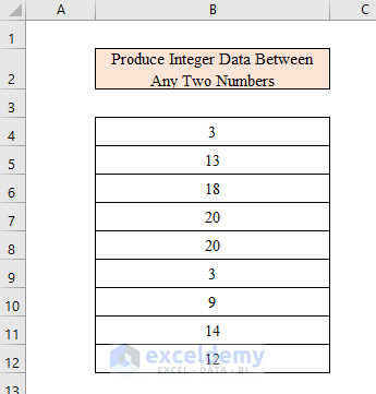
- Press CTRL+Enter.
This is the output.
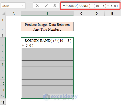
This same method can be applied to negative numbers. To generate random integer data between -5 to 10.
Step 2:
- Select cells.
- Use the formula.
= ROUND( RAND( ) * ( 10 - -5 ) + -5, 0 )
The ROUND function rounds up to the nearest integer.
The RAND function produces a random number between the upper and lower values.
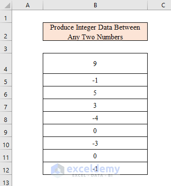
- Press CTRL+Enter to see the result.
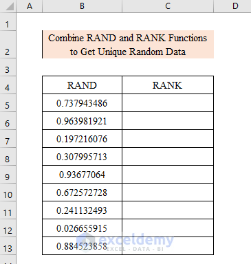
Method 3 – Combining the RAND and the RANK Functions to Get Unique Random Data
Step 1:
- Select cells to enter random data.
- Enter the formula.
=RAND()The RAND function returns a random number between 0 and 1.
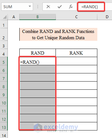
- Press CTRL+Enter.
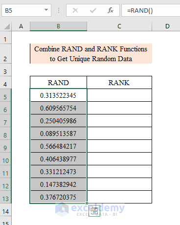
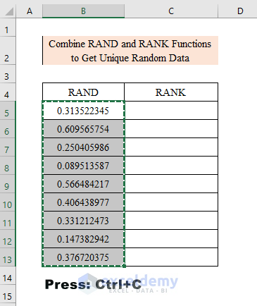
Step 2:
- Select the output of the RAND function.
- Press: CTRL+C.
- Right-click and paste the values.
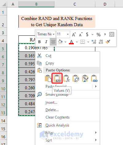
This is the output.
Step 3:
- Select a new column to get unique data.
- Enter the formula
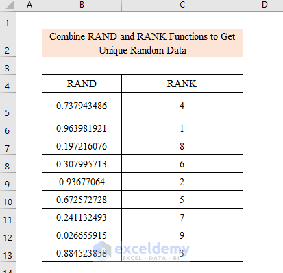
=RANK.EQ(B5,$B$5:$B$13)
The RANK.EQ function returns the rank of a number against a list of other numeric values.
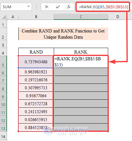
- Click CTRL+Enter.
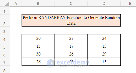
Method 4 – Using the RANDARRAY Function to Generate Random Data in Excel
Steps:
- Select a range to enter random data.
- Enter the following formula.
=RANDARRAY(4,3,10,30,TRUE)The RANDARRAY function returns an array of random numbers between 0 and 1.
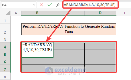
- Click CTRL+Enter.
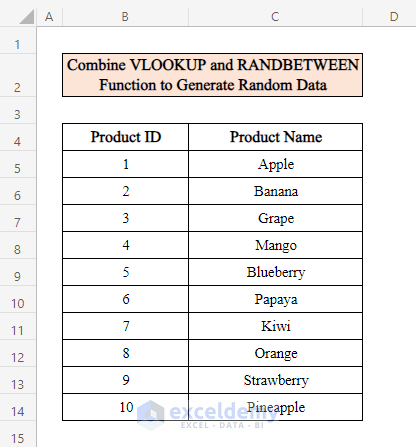
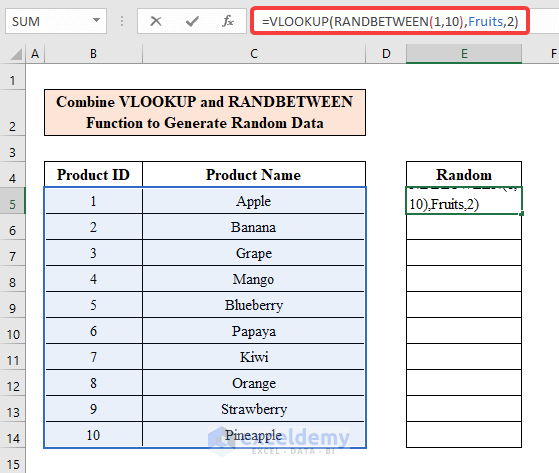
Method 5 – Combining the VLOOKUP and the RANDBETWEEN Functions to Generate Random Data in Excel
The dataset of a fruit shop contains Product ID and Product name.
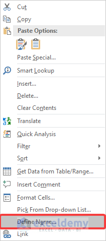
Step 1:
- Select the dataset and right-click.
- In the options box, select “Define Name”.
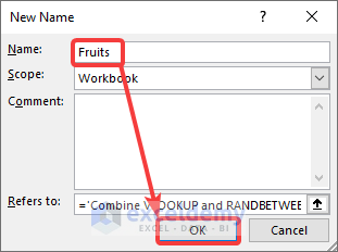
Step 2:
- In the “New Name” window, enter Fruits in “Name”.
- Click OK.
Step 3:
- Select a column to display random fruit names.
- Enter the formula.
=VLOOKUP(RANDBETWEEN(1,10),Fruits,2)
The RANDBETWEEN function distributes data within the given upper and lower values.
The VLOOKUP function searches for a value and returns it from a different column in the same row.
- Press CTRL+Enter.
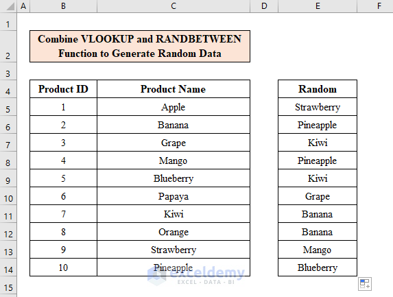
- Drag down the Fill Handle to get random fruit names in the column.
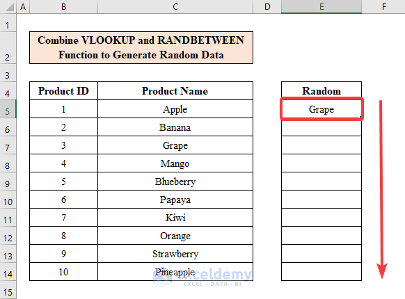
This is the output.
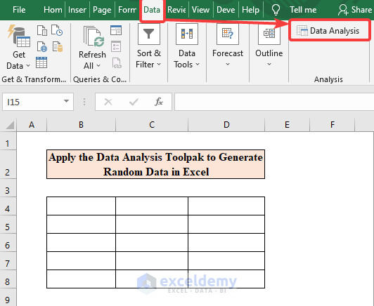
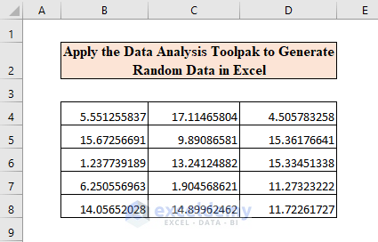
Method 6 – Applying the Data Analysis Toolpak to Generate Random Data in Excel
Step 1:
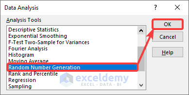
- Choose “Data” on the ribbon and go to “Data Analysis”.
- In the” Data Analysis” window, select “Random Number Generation” in Analysis Tools.
- Click OK.
Step 2:
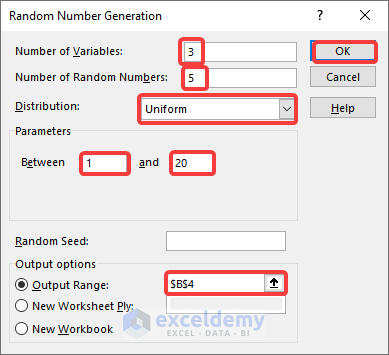
- In the window “Random Number Generation” enter a “Number of Variables” and a “Number of Random Numbers”.
Number of Variables indicates the number of columns you want to add.
Number of Random Numbers indicates the number of data in each column.
- In the drop-down list select “Uniform”.
- Choose the Parameters. Here, between 1 and 20.
- Click “Output Range” and select a cell in the workbook.
- Click OK.
This is the output.
Method 7 – Running a VBA Code to Generate Random Data in Excel
Step 1:
- Press: ALT+F11 to open up the VBA Editor.
- Go to Insert > Module.
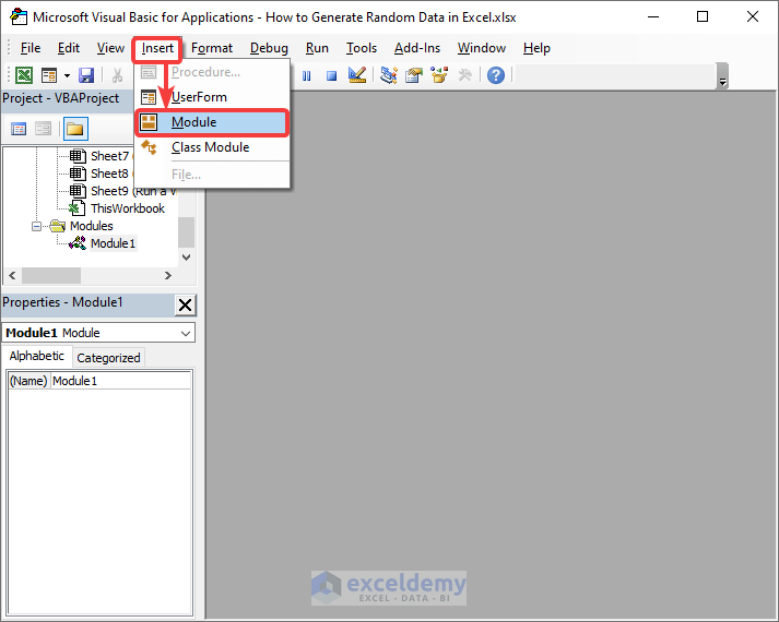
- In the Module window, enter the code-
Sub Randomdata()
     MsgBox Rnd()
End Sub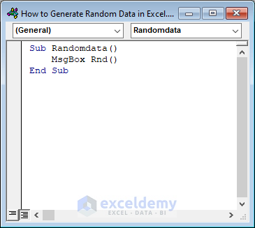
- Run the code.
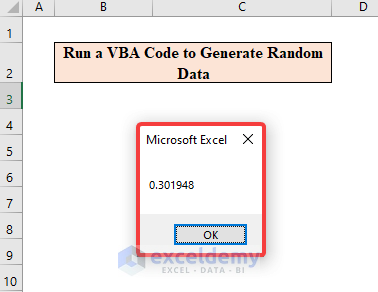
- You will see random decimal numbers.
To round values:
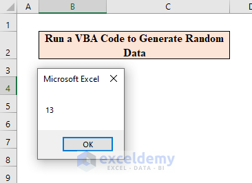
Step 2:
- Select “Module” in “Insert”.
- Enter the following code in the module window.
Sub Randomdata()
 MsgBox Round((Rnd() * 10) + 5)
 End Sub
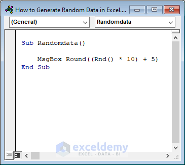
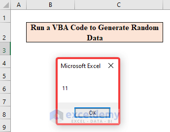
- Click Run.
This is the output.
To display your random data in a grid.
Step 3:
- In the Module window enter the code-
Sub RandomNumber()
 Dim I As Integer For I = 1 To 5
   Cells(I, 1) = Round((Rnd(10) * 10) + 5, 0)
 Next I
 End Sub
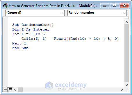
- Run the macro.
- This is the output.
Method 8 – Merging the RANK.EQ and the COUNTIF Functions to Generate Random Data without Duplicates
Step 1:
- Select cells in a column. Here, B4:B13.
- Enter the formula-
=RANDBETWEEN(1,20)
The RANDBETWEEN function calculates a random number between two numbers.
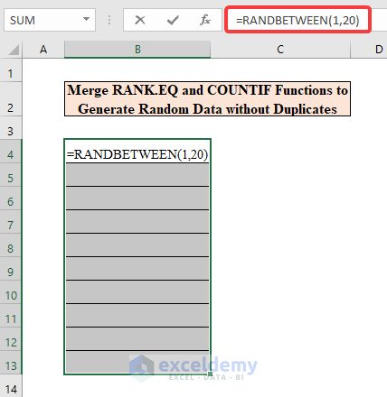
- Press CTRL+Enter to generate random data between 1 to 20.
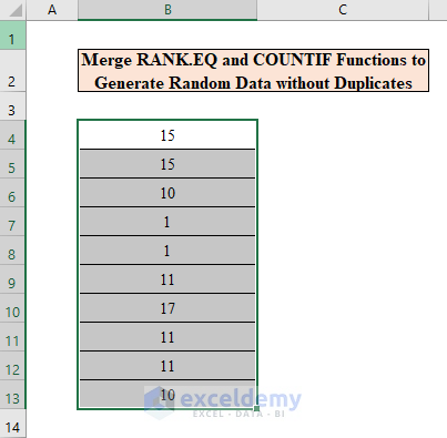
To find duplicate numbers:
Step 2:
- Select the cells.
- Press CTRL+C to copy.
- Right-click and in Paste, select Values.
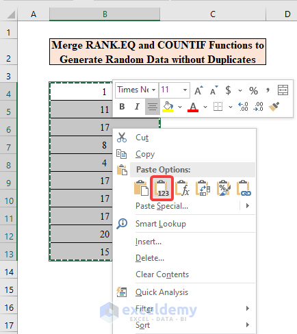
This is the output.
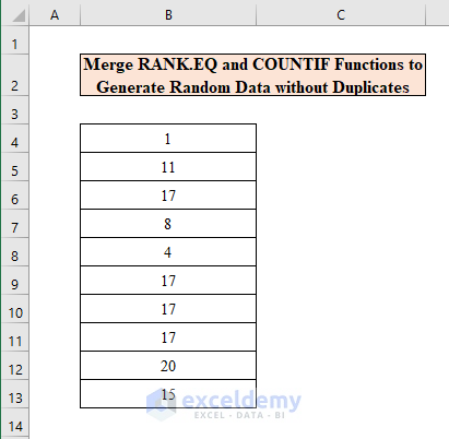
To get unique values only.
Step 3:
- Select a new column to display unique data.
- Enter the formula.
=RANK.EQ(B4,$B$4:$B$13)+COUNTIF($B$4:B4,B4)-1
The EQ function calculates and returns the statistical rank of a given value.
The COUNTIF function counts the number of cells in a given range.
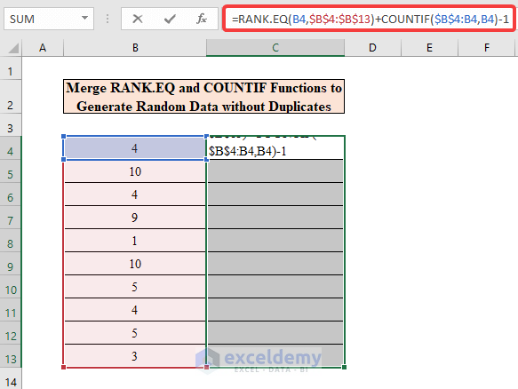
- Press CTRL+Enter.
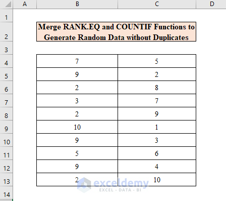
This is the output.
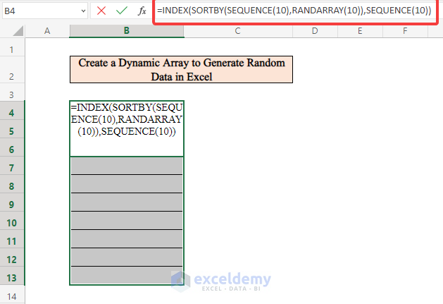
Method 9 – Creating a Dynamic Array to Generate Random Data in Excel
Steps:
- Select B4:B13.
- Enter the formula.
=INDEX(SORTBY(SEQUENCE(10),RANDARRAY(10)),SEQUENCE(10))
The INDEX function returns the value at a given location in an array.
The SORTBY function sorts the data in an array.
The SEQUENCE function generates a list of sequential numbers.
The RANDARRAY function returns random numbers between 0 and 1.
- Press CTRL+Enter.
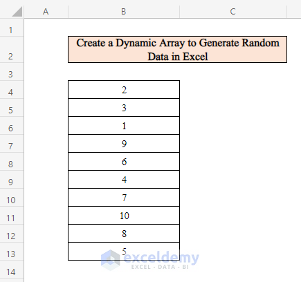
This is the output.
Things to Remember
- When applying the “Data Analysis” ToolPak method, you may need to install it:
File > Options > Select “Analysis Toolpak” from “Add-ins” window > OK > Put Tick in the “Analysis Toolpak” > OK.
- The RANDARRAY and the SORTBY functions are only available in Excel 365.
- After getting the random data don’t forget to convert it into values. Otherwise, data will keep changing.
Download Practice Workbook
Download this practice workbook to exercise.
<< Go Back to Random Number in Excel | Randomize in Excel | Learn Excel
Get FREE Advanced Excel Exercises with Solutions!
