Introduction to ROUND Function
Function Objective
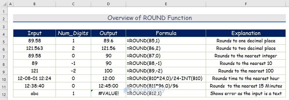
The ROUND function is a powerful tool for rounding numbers based on a specified number of digits. Whether you need to round up or round down, this function has you covered.
Syntax
The syntax for the ROUND function is as follows:
=ROUND (number, num_digits)Arguments Explanation
| Arguments | Required/Optional | Explanation |
|---|---|---|
| number | required | The value you want to round. |
| num_digits | required | The number of decimal places to which you want to round the numeric argument. |
Return Value
The ROUND function provides a rounded numerical value.
Note
- When the number of digits is between 1 and 4, the ROUND function rounds down. For 5 to 9 digits, it rounds up.
- To always round up, consider using the ROUNDUP function. Conversely, the ROUNDDOWN function always rounds down.
- The number of digits significantly affects the output. Let’s explore the different forms of rounding:
| Number of Digits | Forms of Rounding |
|---|---|
| >0 | Rounds to the decimal point |
| 0 | Rounds to the nearest integer |
| <0 | Rounds to the nearest 10, 100, etc. |
Dataset Overview
Here’s an overview of the dataset that we’ll use in our examples.
Example 1 – Positive Number of Digits
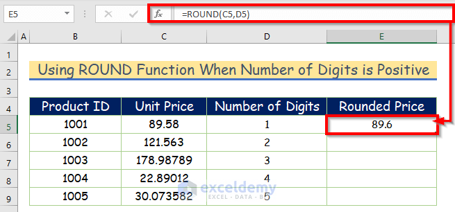
Suppose you have a dataset with unit prices, and you want to round them based on the number of digits. Let’s say the unit price is in cell C5, and the number of digits is in cell D5. Here’s how you can do it:
- Select cell E5.
- Enter the following formula:
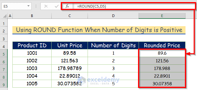
=ROUND(C5,D5)- Press Enter. The result in cell E5 will be 89.6.
- AutoFill the formula to the rest of the cells in column E.
Example 2 – Negative Number of Digits
When the number of digits is negative, the ROUND function rounds to the nearest multiple of 10, 100, etc. Repeat the same method as in Example 1.
=ROUND(C5,D5)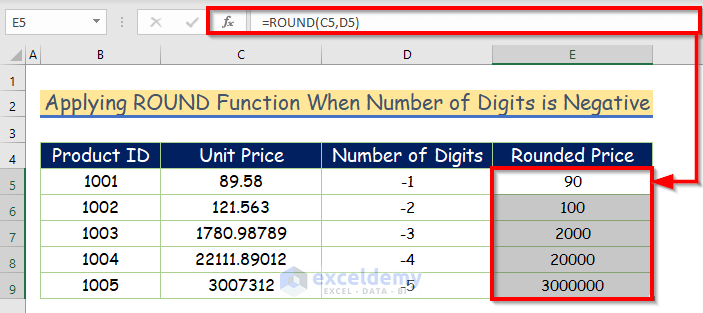
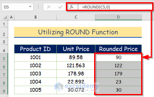
Example 3 – Nearest Whole Number
For zero digits, the ROUND function rounds to the nearest whole number. Follow these steps:
- Select cell D5.
- Enter the formula:
=ROUND(C5,0)
- Press Enter. The output in cell D5 will be 90.

- AutoFill the formula to the rest of the cells in column D.
Example 4 – Rounding to Two Decimal Places
To round a number to two decimal places, enter the formula:
=ROUND(C5,2)Where C5 is the number, and 2 represents the desired decimal places.

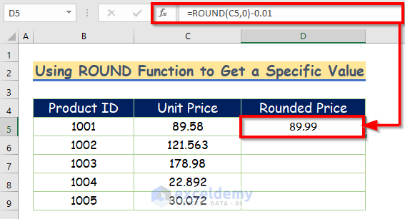
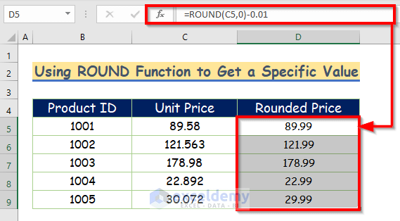
Example 5 – Specific Rounded Value
Suppose you need a specific rounded value, such as rounding to the nearest 0.99. Follow these steps:
- Select cell D5.
- Enter the formula:
=ROUND(C5,0)-0.01Formula Breakdown
- ROUND(C5,0) rounds to the 90.
- After subtracting 01, you’ll get the desired number.
- Press Enter and the result will be 89.99.
- AutoFill the formula to the rest of the cells in column D.
Example 6 – Rounding Up to Nearest 10/100/1000
i. Round Up to the Nearest 10
To find the rounded number to the nearest multiple of 10, enter the following formula:
=ROUND(C5,-1)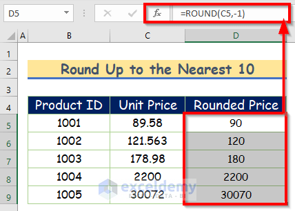
ii. Round Up to the Nearest 100
For rounding to the nearest multiple of 100, enter:
=ROUND(C5,-2)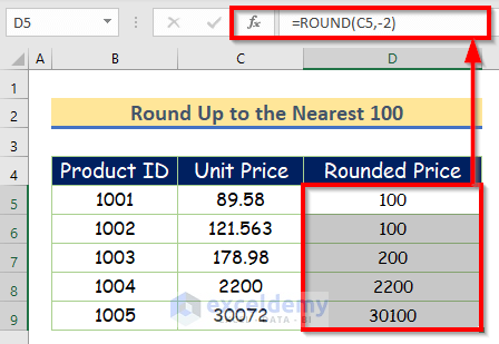
iii. Round Up to the Nearest 1000
To calculate the rounded number to the nearest 1000 (or a multiple of that), enter:
=ROUND(C5,-3)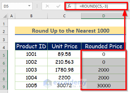
Example 7 – Rounding Time in Excel Using the ROUND Function
You can also apply the ROUND function to time values. Since Excel stores dates and times as serial numbers, the function calculates time as a serial number. To display the result as time, follow these steps:
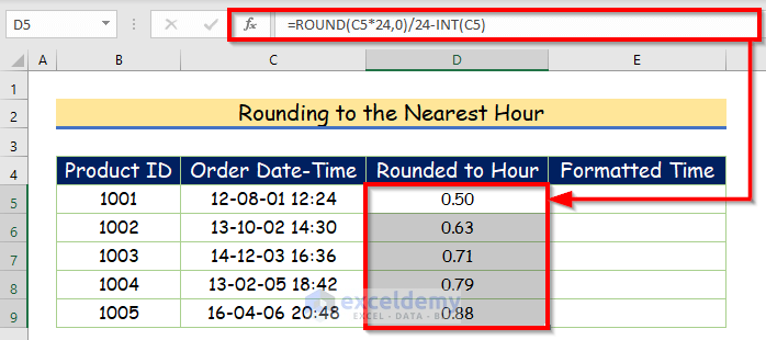
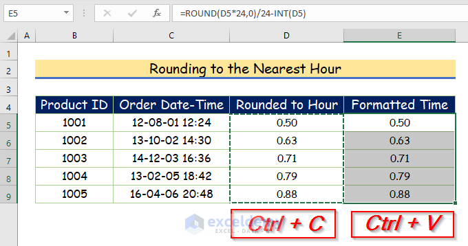
i. Rounding to the Nearest Hour
A day has 24 hours, thus the formula will be:
=ROUND(D5*24,0)/24-INT(D5)Here, the INT function subtracts the date portion.
- Format the fraction values as shown in the screenshots below:
(Note: Images are for illustrative purposes only)
- Select the cells from D5 to D9 and copy this range using the Ctrl + C keyboard shortcut. Paste the copied portion using the Ctrl + P simultaneously.
- Select the cells from E5 to E9 and press Ctrl + 1 simultaneously.
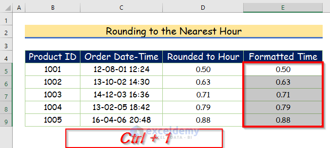
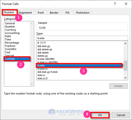
- A Format Cells dialog box will pop up.
- From the Format Cells dialog box, select Number.
- Under Category, select Custom and select h:mm as Type.
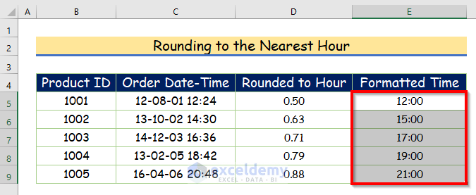
- The fraction values have been formatted into h:mm format.
ii Rounding to the Nearest 15 Minutes
Since a day has 96 intervals of 15 minutes each, enter:
=ROUND(C5*96,0)/96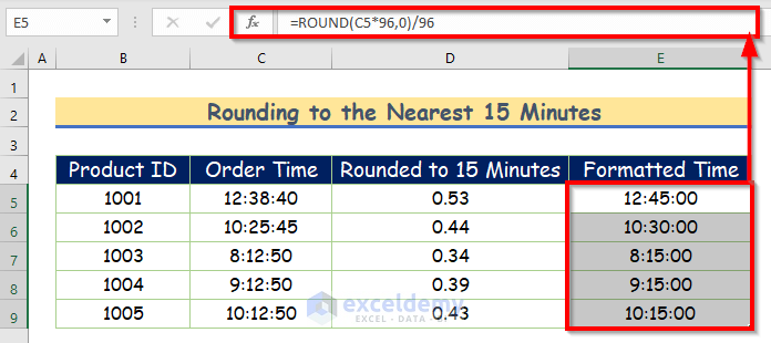
Example 8 – Rounding the Total of Two Numbers
Consider two numbers (e.g., price in June and price in July). To find the rounded total value, enter:
=ROUND(C5+D5,0)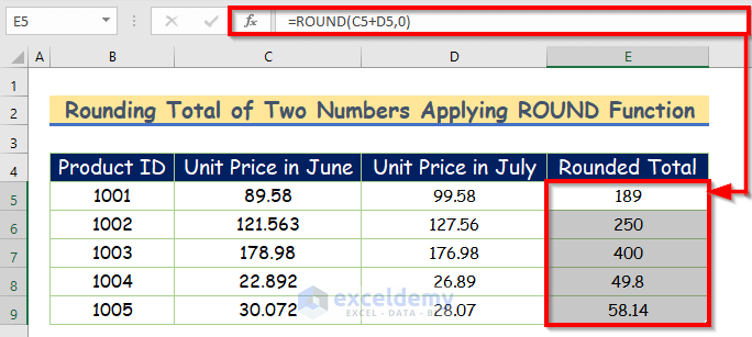
Example 9 – Rounding the Quotient of Two Numbers
For the quotient of two numbers, enter:
=ROUND(D5/C5,0)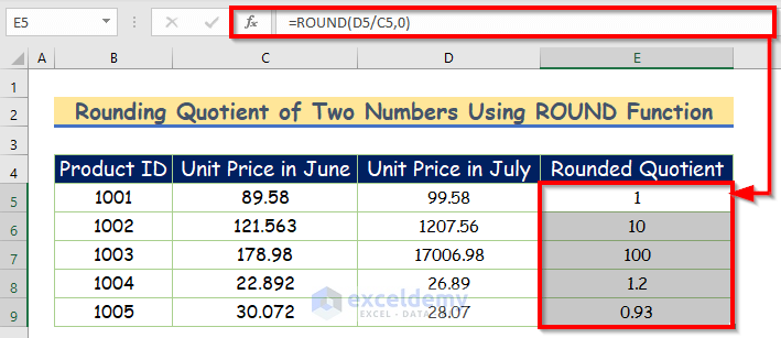
Common Errors While Using ROUND Function
- Remember that the #VALUE! error occurs when text is inserted as input.
Download Excel Workbook
You can download the practice workbook from here:
<< Go Back to Excel Functions | Learn Excel
Get FREE Advanced Excel Exercises with Solutions!
