What Is Drop Down List?
A drop-down list allows the user to choose text or numbers from a list rather than typing them into a cell.
To insert a drop-down list:
- Select the cells where the drop-down lists are needed.
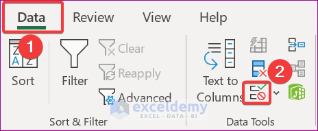
- Go to the Data tab.
- Click the Data Validation option in the Data Tools group.
- Check the List option in the Validation criteria in the Data Validation window.
Excel Drop Down List Ignore Blank Not Working: 3 Solutions
Whenever we try to create a drop-down list in a range that contains blank cells, the list will include an empty option. Attempting to use the Ignore Blank option will not prevent this. In this article we will demonstrate three solutions to remove these empty cells from the drop-down menu.
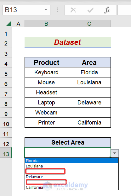
To demonstrate our methods, we’ll use a sample dataset containing two columns titled Product and Area.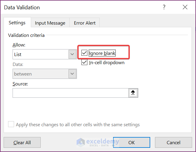
We used the Microsoft Excel 365 version here, but you can use any version available to you.
Reason – Source Range of Drop Down List Contains Blank Cells
When there are empty cells in the Source Range, after creating a drop-down list using the Data Validation feature as described above, some items remain blank while displaying the list.
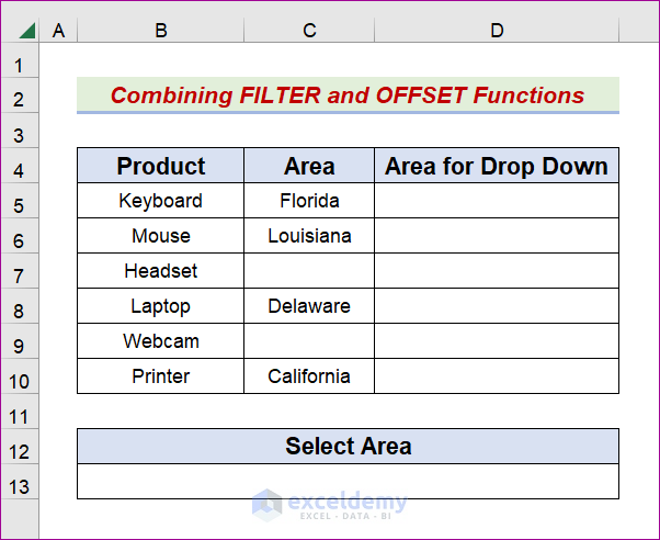
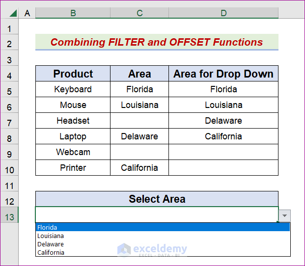
Solution 1 – Using FILTER and OFFSET Functions
We can use the FILTER and OFFSET functions to remove the empty cells from a drop-down menu.
Steps:
- Create a column titled Select Area like the below one.
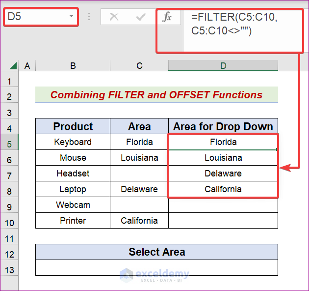
- In cell D5, enter the following equation:
=FILTER(C5:C10,C5:C10<>"")
- Press Enter or Tab to return the result.
- Navigate to the Formulas tab and click on the Name Manager icon.
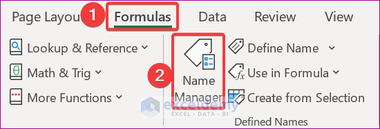
- In the Name Manager window that appears, click New.
![]()
The New Name window will open.
- Enter the name, in this case DropDownWithoutBlank.
- Enter the following formula in the Refers to box:
=OFFSET(OFFSETFunction!$D$5,0,0,COUNTA(OFFSETFunction!$D$4:$D$10)-1,1)
- Click OK.
![]()
- Choose Close from the Name Manager window.
![]()
- Select cell B13.
![]()
- Go to the Data tab and click on the Data Validation symbol.
The Data Validation window will pop up.
- From the Settings tab, choose List in the Allow box.
- In the Source box, enter an Equal sign followed by the Range name created earlier.
- Click OK.
![]()
After expanding it, the drop-down list will display without the blanks.
Read More: How to Remove Used Items from Drop Down List in Excel
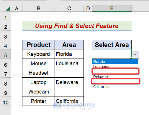
Solution 2 – Using the Find & Select Feature
Steps:
- Make another column named Select Area.
- Select cell E5.
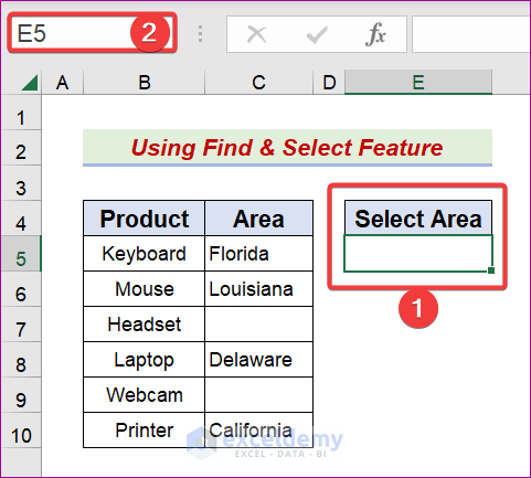
- Navigate to the Data tab and click on the Data Validation icon.

The Data Validation dialog box will appear.
- From the Settings tab, choose List in the Allow section.
- Input an Equal sign followed by the $C$5:C$10$ range and click OK.
![]()
After expanding it, the drop-down will display a drop-down with some empty cells.
- To eliminate those, select the C5:C10 range.
![]()
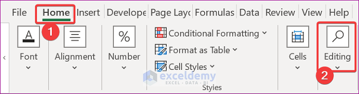
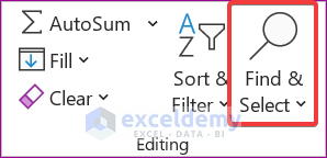
- Go to the Home tab and click on Editing.
- From the Editing group, choose Find & Select.
- Pick the Go To Special option.
![]()
- From the Go To Special window, check Blanks and click OK.
![]()
The outcome will look like the below.
![]()
- Right-click on any selected empty cell and from the Context menu, choose Delete.
![]()
- Check the Shift cells up option and click OK.
![]()
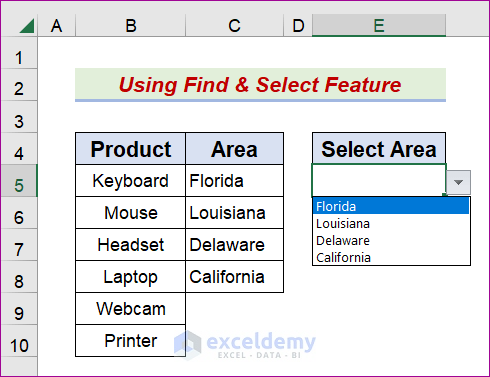
- The desired outcome will be produced.
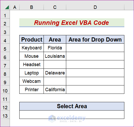
Solution 3 – Using Excel VBA Code
Steps:
- Make another column titled Select Area.
- Go to the Developer tab and choose the Visual Basic symbol.

- Click on Insert >> Module.
Insert → Module
![]()
- Enter the code below in the Module box that opens:
Sub DropDownWithNoBlank()
    Range("D5").Select
    ActiveCell.Formula2R1C1 = "=FILTER(RC[-1]:R[5]C[-1],RC[-1]:R[5]C[-1]<>"""")"
    ActiveWorkbook.Names.Add Name:="DropDownWithoutBlankUsingExcelVBA", _
        RefersToR1C1:= _
        "=OFFSET(OFFSETFunction!R5C4,0,0,COUNTA(OFFSETFunction!R4C4:R10C4)-1,1)"
    Range("B13:D13").Select
    With Selection.Validation
        .Delete
        .Add Type:=xlValidateList, AlertStyle:=xlValidAlertStop, Operator:= _
        xlBetween, Formula1:="=DropDownWithoutBlankUsingExcelVBA"
        .IgnoreBlank = True
        .InCellDropdown = True
        .ShowInput = True
        .ShowError = True
    End With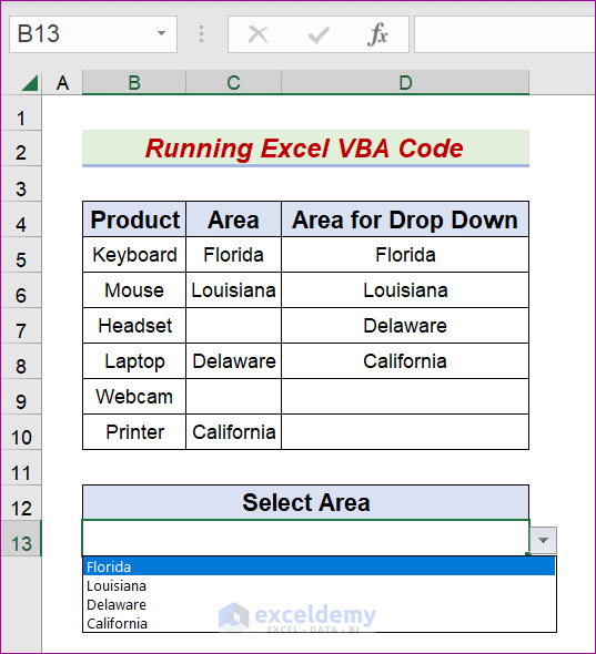
End Sub- Press F5 or click on the Run button to run the code.
![]()
The drop-down displays without blanks.
Read More: Hide or Unhide Columns Based on Drop Down List Selection in Excel
Download Practice Workbook
Related Articles
- How to Create Drop Down List in Multiple Columns in Excel
- Create a Searchable Drop Down List in Excel
- Creating a Drop Down Filter to Extract Data Based on Selection in Excel
- How to Select from Drop Down and Pull Data from Different Sheet in Excel
- How to Create a Form with Drop Down List in Excel
- How to Remove Duplicates from Drop Down List in Excel
- How to Fill Drop-Down List Cell in Excel with Color but with No Text
- How to Make Multiple Selection from Drop Down List in Excel
- How to Autocomplete Data Validation Drop Down List in Excel
<< Go Back to Excel Drop-Down List | Data Validation in Excel | Learn Excel

