Hide or Unhide Columns Based on Drop Down List Selection in Excel

This article illustrates several examples to hide or unhide columns in Excel based on drop–down list selection. We’ll use VBA code to first set conditions to select columns and then hide or unhide them based on those conditions. Let’s dive into the examples to get a clear understanding of the whole procedure.

Download Practice Workbook

Download this practice workbook to exercise while you are reading this article.

2 Examples to Hide or Unhide Columns Based On Drop Down List Selection in Excel

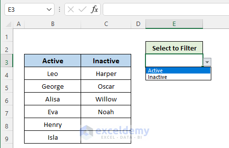
At first, we need to create a drop-down list with the help of the dataset. The drop-down list would hold the options based on which we’ll hide or unhide columns. Let’s say we have a list of active and inactive members of a sports club. We want to make a drop-down list with two options– active and inactive and then hide and unhide those columns based on the selection.

Create a Drop-Down List in Excel:

To make a drop–down list, just follow the simple steps below-

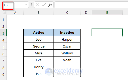
• Select a cell (E3, in this example) on which we’ll create the drop-down list.

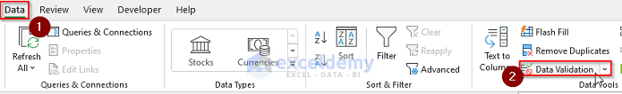
• Then go to the Data tab of the Excel Ribbon.
• Click on the Data Validation option.

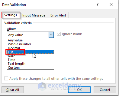
• In the Data Validation window, select the Setting tab (By default get selected).
• In the Allow drop-down list, choose the List option.

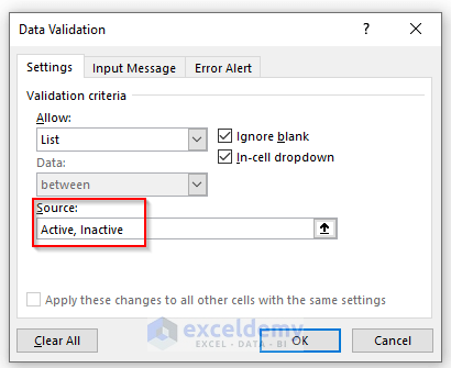
• Then type Active and Inactive in the Source input box and finally hit OK.

• As an output, we can see a drop-down list in cell E3 with two options to select- Active and Inactive.

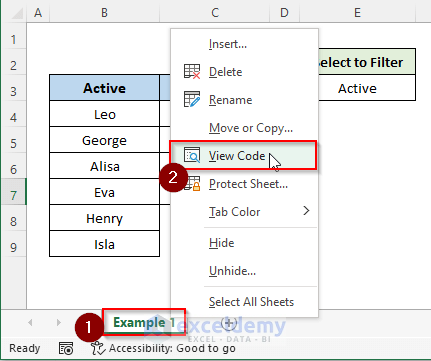
Example 1: Hide or Unhide Columns Based On Drop Down List Selection in Excel

In this example, we’ll work on the dataset we discussed earlier to filter the active and inactive members by using the drop–down list. On the selection of the Active option, we want to hide the column with inactive members and vice versa. To do that let’s follow the steps described below-

• Right-click on the sheet name and select the View Code option.

• Then copy and paste the following code in the visual code editor.

Private Sub Worksheet_Change(ByVal Target As Range)
    If Target.Address = ("$E$3") Then
        If Target.Text = "Active" Then
            Columns("C").EntireColumn.Hidden = True
            Columns("B").EntireColumn.Hidden = False
        ElseIf Target.Text = "Inactive" Then
            Columns("C").EntireColumn.Hidden = False
            Columns("B").EntireColumn.Hidden = True
        End If
    End If
End Sub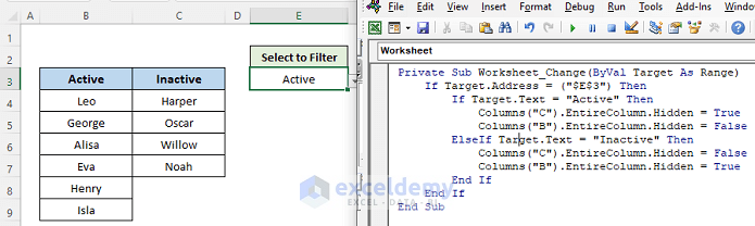

• Save the code by pressing Ctrl + S and then close the code editor.
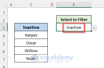
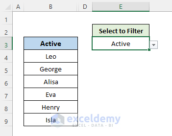
• Now on the worksheet, to hide the active members’ column e., keeping only the inactive members’ column, choose the Inactive option from the drop–down list.

• Again, we selected the Active option from the drop-down list.

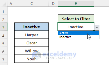
• This time the column with active members appeared and the column with inactive members got hidden.

Code Explanation:

In our code,

• we used the EntireColumn property to select the entire column with active and inactive members.
• Then we set the .hidden property to True or False to hide a specific column.

Read More: How to Make Multiple Selection from Drop Down List in Excel (3 Ways)

Similar Readings:

• How to Create Dependent Drop Down List with Multiple Words in Excel
• How to Remove Duplicates from Drop Down List in Excel (4 Methods)
• Create a Searchable Drop Down List in Excel (2 Methods)
• How to Add Blank Option to Drop Down List in Excel (2 Methods)
• How to Change Drop Down List Based on Cell Value in Excel (2 Ways)

Example 2: Hide or Unhide Columns to Filter Data Based On Drop Down List Selection in Excel

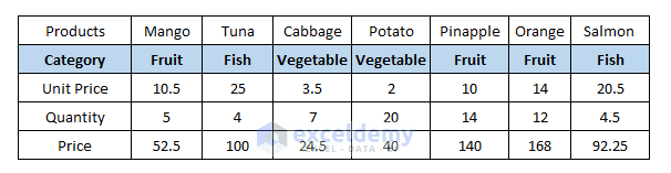
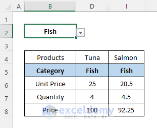
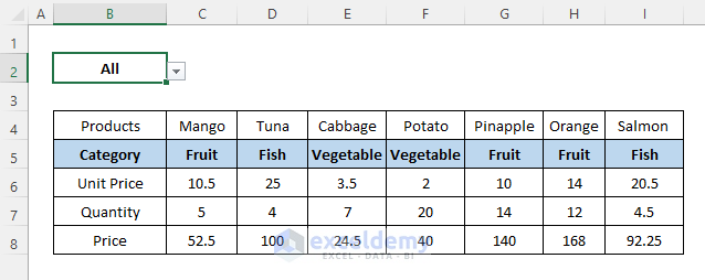
In this example, we’re going to filter a sale list based on category selection. The sale list contains sales data for 7 products from 3 different categories i.e., Fruit, Vegetable, and Fish.

We want to hide all other columns except the columns with the selected category in the drop-down. In addition, all the columns will be visible when we’ll select the All option from the drop-down. To accomplish the task let’s follow the steps below.

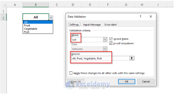
• In cell B2, create a drop-down list with 4 options- All, Fruit, Vegetable, and Fish. For this follow the steps in the Create a Drop-Down List in Excel section that is described earlier in the article.

• Now to open the Visual Code Editor, right–click on the sheet name and choose the View Code option.

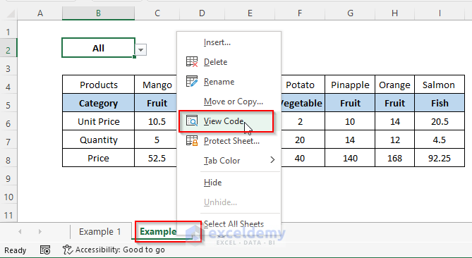
• Copy and paste the following code into the editor.

Option Explicit
Private Sub Worksheet_Change(ByVal Target As Range)
    Dim a As Variant, b As String
     If Target.Column = 2 And Target.Row = 2 Then
        b = Target.Value2
        With Range("C5:I5")
            Application.ScreenUpdating = False
            .EntireColumn.Hidden = (b <> "All")
            If b <> "All" Then
                For Each a In .Cells
                    If a = b Then a.EntireColumn.Hidden = False
                Next
            End If
            Application.ScreenUpdating = True
        End With
    End If
End Sub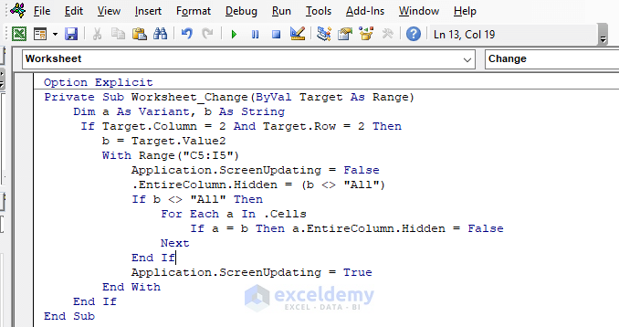

• Save the code by pressing Ctrl + S and then close the code editor.
• Now our dataset is filterable based on the category we select from the drop–down list. The following screenshots are showing the outputs.

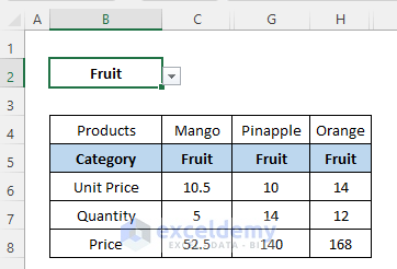
The first image is the list for the Fruit category.

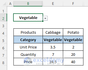
Then we choose the Vegetable category.

The next image shows the Fish category list.

Finally, we choose all the categories.

Code Explanation:

• We selected the target cell B2 using the following line of code defining its column and row number. We did it differently in example 1 using the Address property.

   If Target.Column = 2 And Target.Row = 2 Then

• The variable b holds the value of the selected category in the drop–down.
• The following code defines the range of cells containing category names in the sale list. Each of the values is matched against the variable b.

 With Range("C5:I5")

• If the value of b matches with one of the values of Range(“C5:I5”), the code selects the entire column associated with the cell and keeps it visible by applying the Hidden property to False.

Read More: Excel Drop Down List Depending on Selection

Things to Remember

In the VBA code, we set the Application.ScreenUpdating = False before starting the loop and again changed to Application.ScreenUpdating = True after finishing the loop to get a faster response while changing the selection in the drop-down list.

Conclusion

Now, we know how to hide or unhide columns in Excel based on drop-down list selection with 2 well-explained examples. Hopefully, it’ll certainly help you to use these methods more confidently. Any questions or suggestions don’t forget to put them in the comment box below.

Related Articles

• How to Make a Drop Down List in Excel (Independent and Dependent)
• How to use IF Statement to Create a Drop-Down List in Excel
• Conditional Drop Down List in Excel (Create, Sort and Use)
• How to Create Dynamic Dependent Drop Down List in Excel
• How to Link a Cell Value with a Drop Down List in Excel (5 Ways)