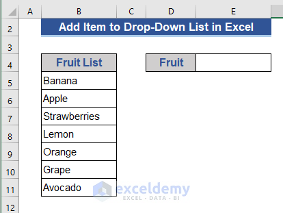
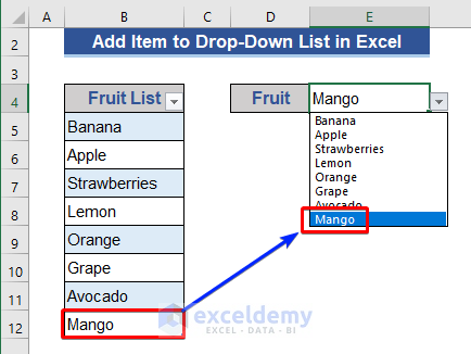
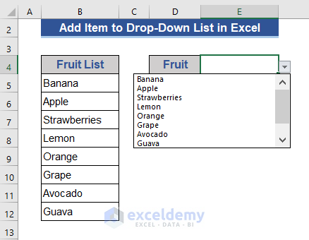
Adding items will depend on how a drop-down list is created. We will consider the following dataset for this purpose.
Method 1 – Add Item to Drop-Down List by Adding Item to Existing Data Range in Excel
Case 1.1 Add Item Within Range Using Insert Feature
Steps:
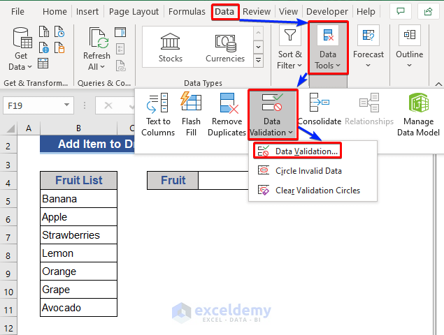
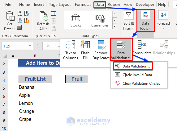
- Move to Cell E4.
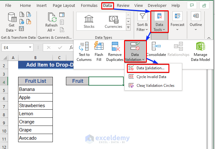
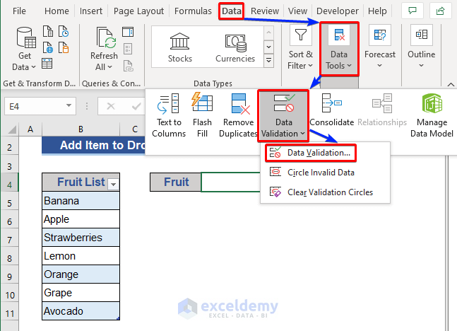
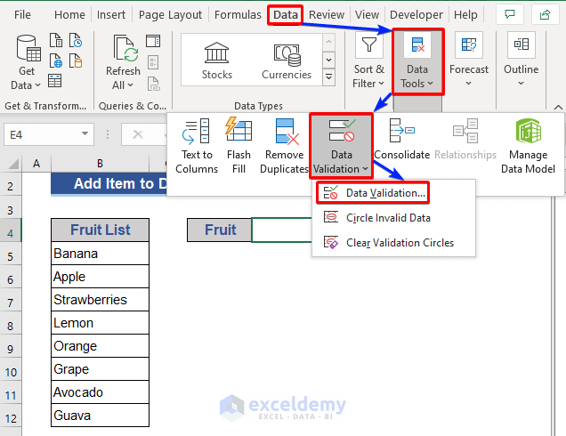
- Select the Data Tools group from the Data tab.
- Choose the Data Validation option.
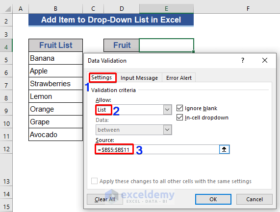
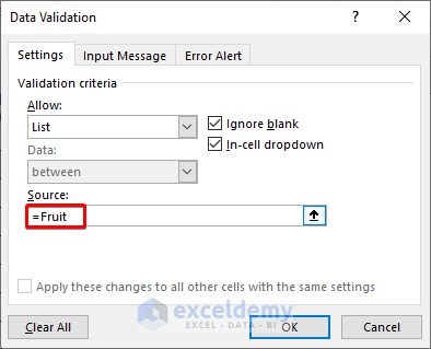
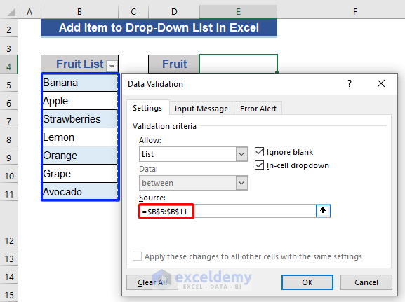
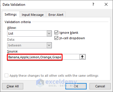
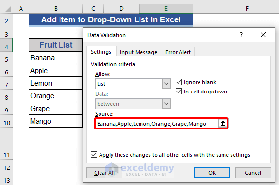
- Choose List from the Allow field.
- Choose the desired range in the Source field and then press OK.
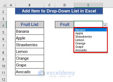
Look at the dataset. The drop-down list is visible at Cell E4.
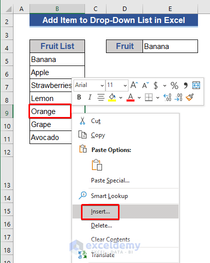
- Move the cursor to any position of the Fruit List column.
- Right-click and choose Insert from the menu.
- Select Shift cells down from the Insert window.
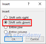
- Press OK.
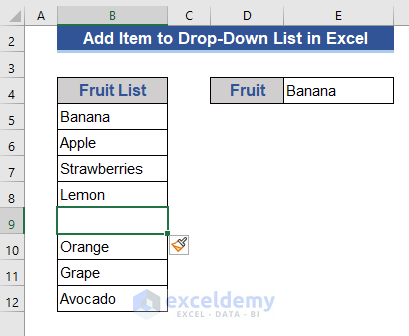
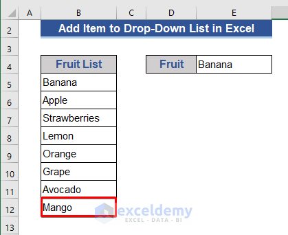
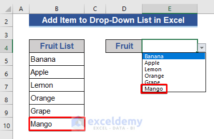
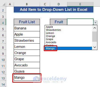
- Write Mango in the empty Cell B9 and click on the drop-down list of Cell E4.
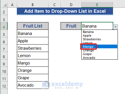
Mango is added to the drop-down list.
Case 1.2 Add Item at the Bottom of Range
Steps:
- Add a new item at the bottom of the Fruit List column.
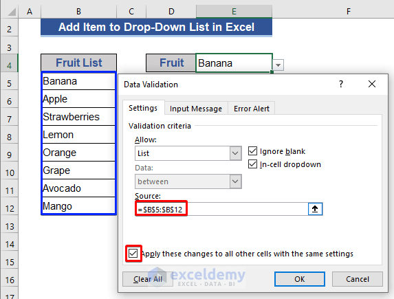
- Go to the Data Validation field by following the steps shown before.
- Modify the Source by selecting the range from the dataset.
- Mark the option Apply these changes to all other cells with the same settings and press OK.
- Move to Cell E4 and click on the down arrow to check the drop-down list.
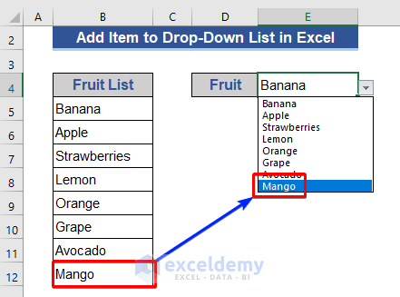
The newly added item is shown on the list.
Method 2 – Add Item to Drop-Down List by Editing a Named Range
Steps:
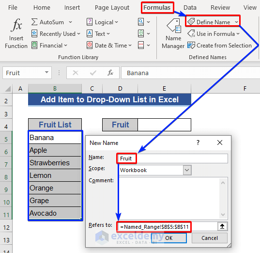
- Select the cells of the Fruit List column.
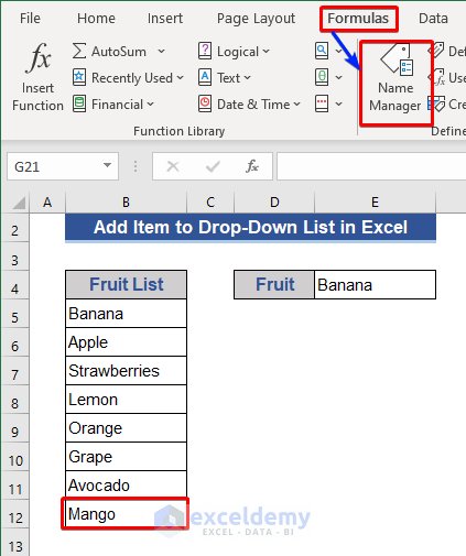
- Select Define Name group from the Formulas tab.
- In the Refers to field, select the range for Named Range.
- Press OK.
- Move the cursor to Cell E4.
- Go to the Data Tools group from the Data tab.
- Select Data Validation from the options and Data Validation from the drop-down.
- The Data Validation window will appear. Put the Named Range title on the Source box.
- Click OK.
Look at the dataset now.
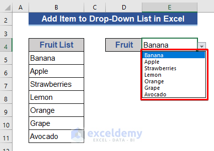
The drop-down list is visible at Cell E4.
We will add new items at the bottom of the dataset and modify the Named Range and that will reflect on the drop-down list.
Steps:
- We added a new item at the bottom of the dataset.
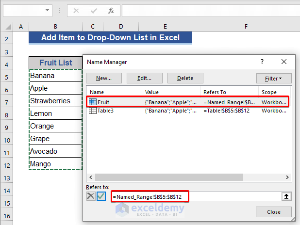
- Go to Name Manager from the Formulas tab.
- In the Name Manager window, go to Refers to select the updated range with newly added data.
- Click Close.
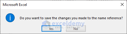
- A new dialog box will appear for permission. Choose Yes.
Go to Cell E4 and click on the down arrow sign.
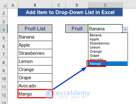
The newly added item is shown on the list.
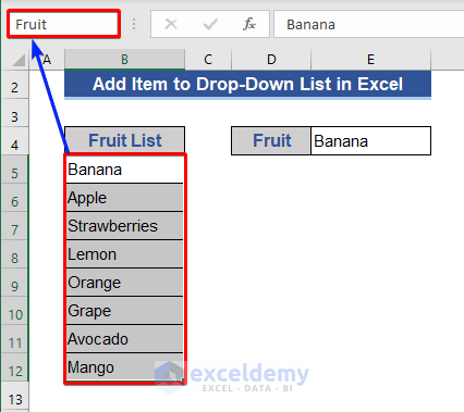
We can apply the Named Range in another simple way. Just select the cells, go to the name bar, and put your desired name.
Read More: How to Edit Drop-Down List in Excel
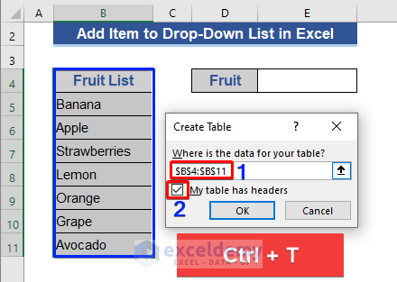
Method 3 – Create a Table-Based Drop-Down List and Add New Item
Steps:
- Select all the cells of the Fruit List.
- Press Ctrl + T.
- The Create Table window will appear. The selected range will show here.
- Mark the box of My table has headers and press OK.
- Move the cursor to Cell E4.
- Go to the Data Tools group from the Data tab.
- Click on the Data Validation option.
- Select the range on the Source field and press OK.
- Click on Cell E4 and press the down arrow sign.
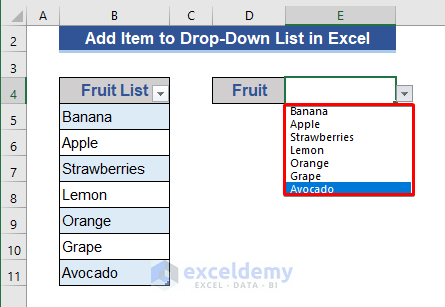
We can see that the drop-down list is visible in the dataset.
- Go to the last cell of the Table.
- Add a new item and press the Enter button.
We can see that the new item is showing on the drop-down list.
Read More: Create Excel Drop Down List from Table
Method 4 – Add Item Manually in an Excel Drop-Down List
Steps:
- Go to Cell E4.
- Go to the Data Tools group from the Data tab.
- Choose the Data Validation option.
- Input 5 items manually on the Source field of the Data Validation option.
- Press OK.
Click on the down arrow of Cell E4.
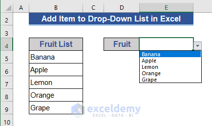
We can see 5 items visible on the drop-down list.
- Go to the Data Validation option again and add a new item to the Source box.
- Mark Apply these changes to all other cells with the same settings option and press OK.
- Go to cell E4.
We can see that the new item is added to the drop-down list.
Method 5 – Add Item by Utilizing Dynamic Drop-Down List in Excel
Steps:
- Select cell E4.
- Choose Data Tools from the Data tab.
- Select the Data Validation option.
- Put the following formula on the Source option.
=OFFSET($B$5,0,0,COUNTA($B:$B),1)
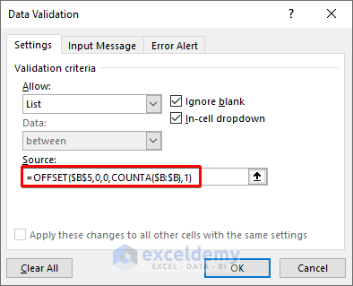
- Press OK.
- Go to cell E4 of the dataset. The drop-down list is visible here.
- Add a new item on the bottom cell of the Fruit List column and press Enter.
Again, go to cell E4 and see that the new item is visible here.
Download Practice Workbook
Download this practice workbook to exercise while you are reading this article.
Related Articles
- How to Create a Drop Down List from Another Sheet in Excel
- How to Remove Drop Down List in Excel
- How to Link a Cell Value with a Drop Down List in Excel
- How to Auto Update Drop-Down List in Excel
- How to Create Excel Drop Down List with Color
- How to Create Drop Down List with Filter in Excel
- How to Create a Drop Down List with Unique Values in Excel
- How to Copy Filter Drop-Down List in Excel
- Excel Drop Down List Not Working
<< Go Back to Edit Drop-Down List in Excel | Excel Drop-Down List | Data Validation in Excel | Learn Excel
Get FREE Advanced Excel Exercises with Solutions!
