How to Link a Cell Value with a Drop Down List in Excel (5 Ways)

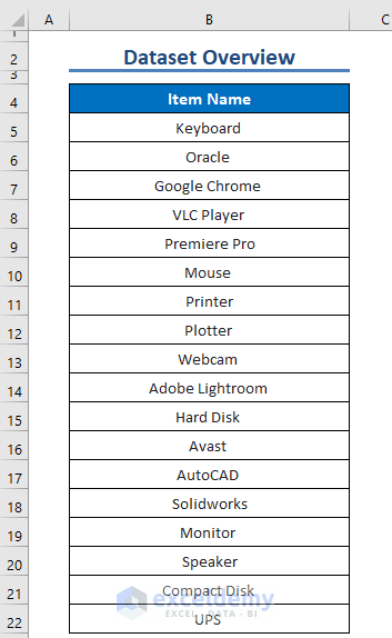
Method 1 – Make a Dynamic Drop-Down List to Link a Cell Value

We have a list of Item Names of some computer accessories. We will make a dynamic drop-down list from it.

Steps:

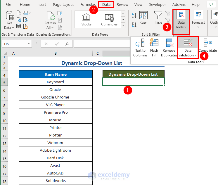
• Select a cell where you want to make the list (i.e. D5).
• Go to the Data tab and click on Data Validation.

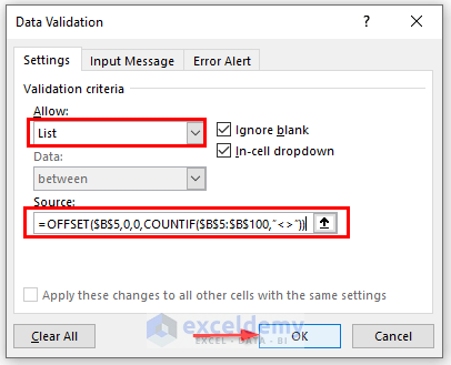
• The Data Validation dialogue box will appear.
• Select “List” as the validation criteria.
• In the source field, insert the following formula:

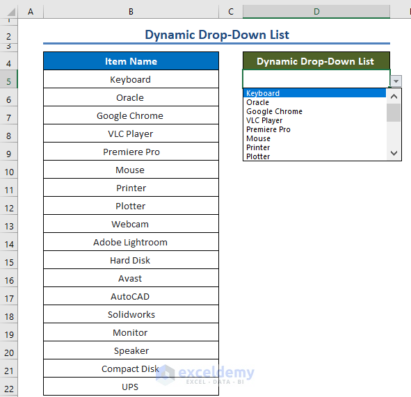
• Click OK to get the drop-down list.

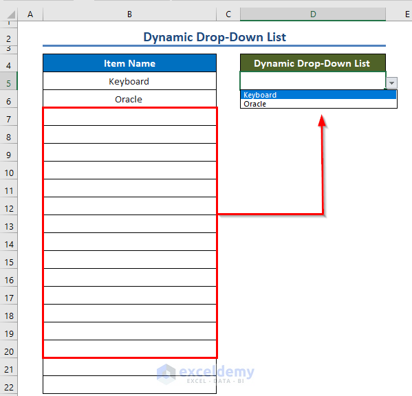
• Delete some data from your data list.
• Open the drop-down list and see that the list has been updated.

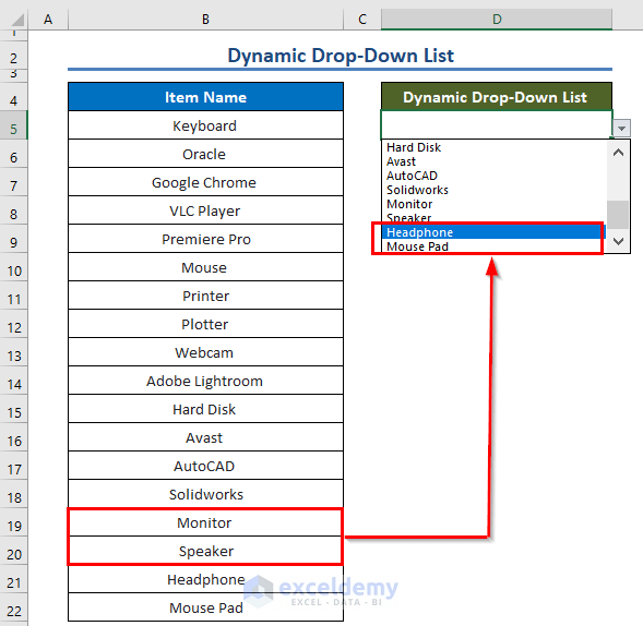
• If we insert some values to the list (by inserting rows in the range), the drop-down will also add these values.

Method 2 – Make a Dependent Drop-Down List to Link a Cell Value

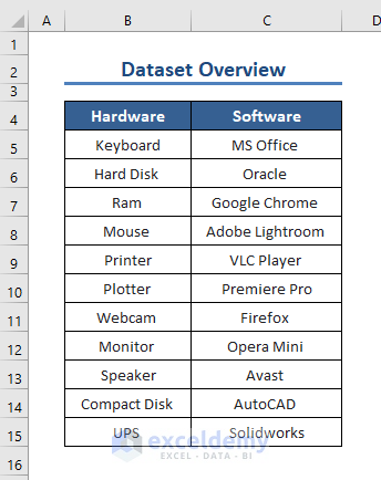
Consider this example where the “Hardware” and “Software” columns are given with some data. We need to make a dependent list, allowing us to select the category and then the item in two lists.

Steps:

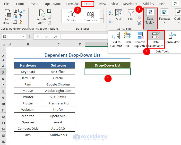
• Select cell E5 and go to the Data tab.
• Select Data Validation from the Data Tools group.

• Select List as validation criteria.
• In the source field, assign the value =$B$4:$C$4.

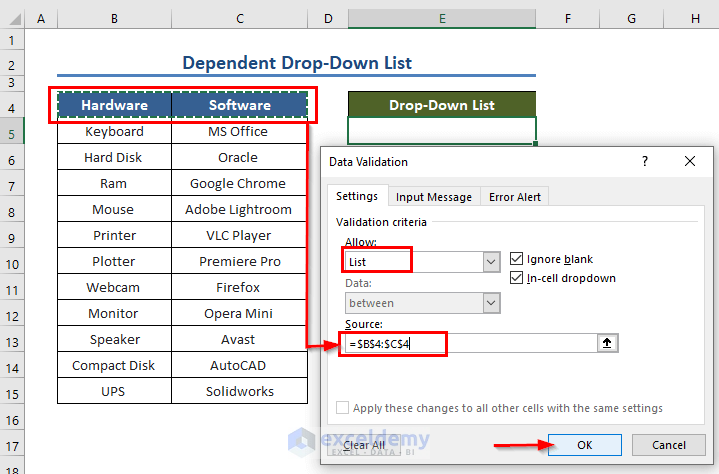
• Click OK to make the list.

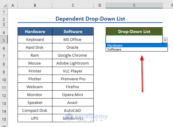
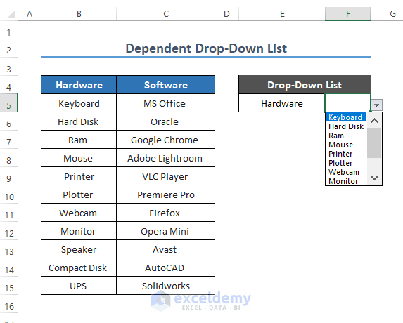
• We have our drop-down list for the columns.
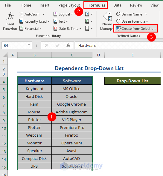
• Select the two original columns.
• Go to Formula and, in the “Name Manager, click on Create From Selection.

• A new window pops out. Check Top Row and click OK.

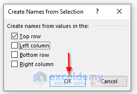
• Click on Close.
• Select cell F4 and go to Data Validation.
• Select List for Allow.
• In the Source box, insert the following:

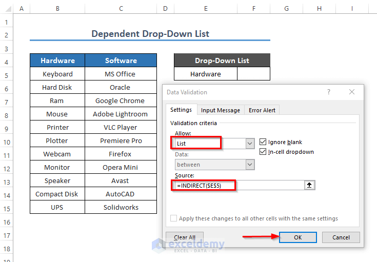
• Click OK.
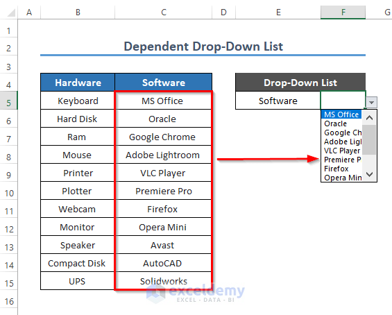
• When you select Hardware in the drop-down list E3, this refers to the named range Hardware (through the INDIRECT function) and thus lists all the items in that category.

• Add or delete values from the source list and the drop-down list will update.

Read More: How to Create Drop Down List with Filter in Excel

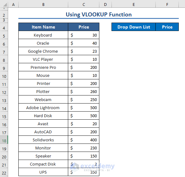
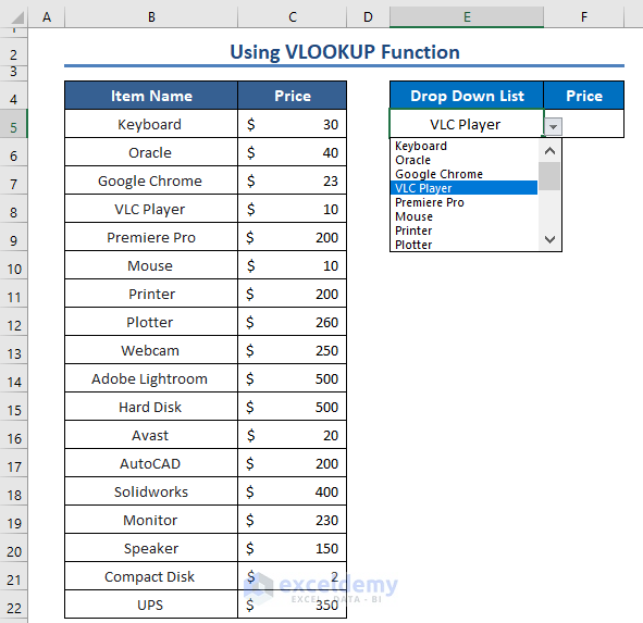
Method 3 – Using the VLOOKUP Function to Link a Cell

We have a list of Item names and their Prices. We will make a drop-down list and link the cell values with the list using the VLOOKUP function.

Steps:

• Make a drop-down list in the cell E5 by following Method 1, using the source data as the cells of the Item Name column.

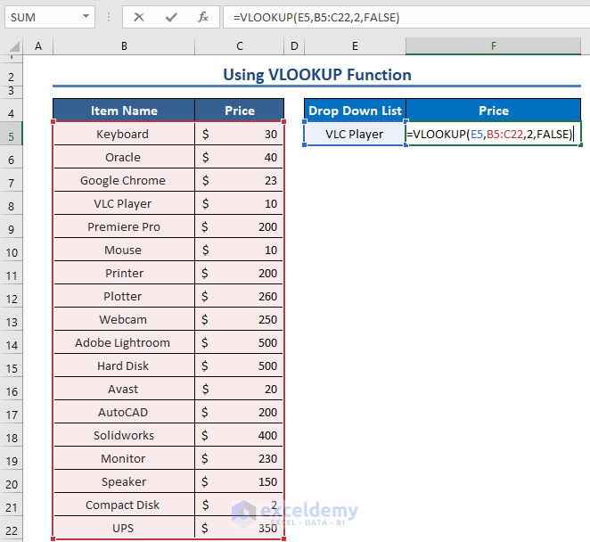
• Apply the VLOOKUP function in the cell F5. The formula is:

• Press Enter.

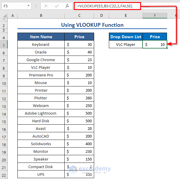
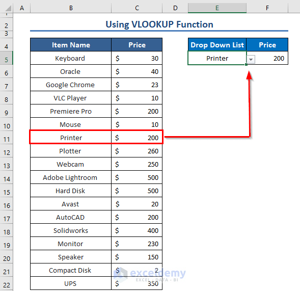
• You can change the list value and check that the cells are linked.

Read More: How to Add Item to Drop-Down List in Excel

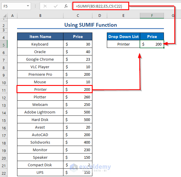
Method 4 – Using the SUMIF Function to Link a Cell

We will use the previous example.

• Create a drop-down for Item Name like in Method 1.
• In the cell F5 apply the following formula:

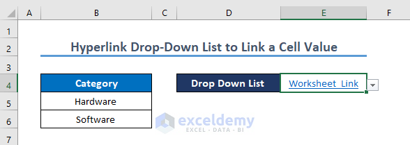
Method 5 – Make a Hyperlink Drop-Down List to Link a Cell Value

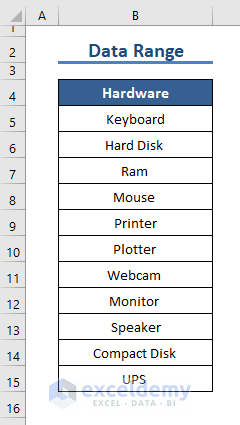
We have two worksheets named Hardware and Software. One of them has data for Hardware.

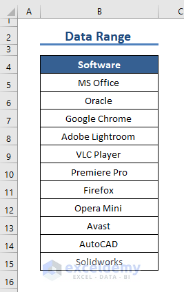
The other contains the data for Software.

Steps:

• Create another worksheet and open it.
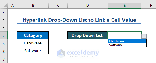
• Make a Category column where you will insert the worksheet name that you want to link with the list.
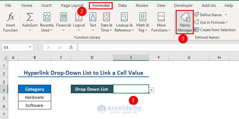
• In cell E4, make the drop-down list for Hardware and Software.

• Select the drop-down list cell, go to Formula, and click on Name Manager.

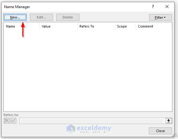
•  Click on New to give this cell a new name.

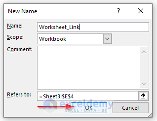
• Name the E4 cell Worksheet_Link and click OK.

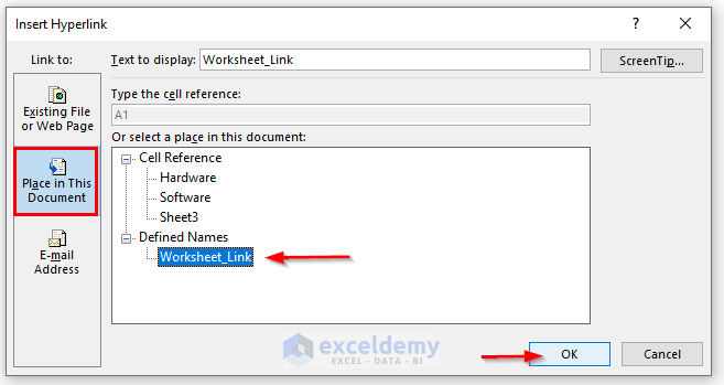
• Select cell E4 and press CTRL + K to create a link in this cell.
• In the new window, select Place in the Document, click on Worksheet_Link, and press OK.

• We will edit the link of this cell.

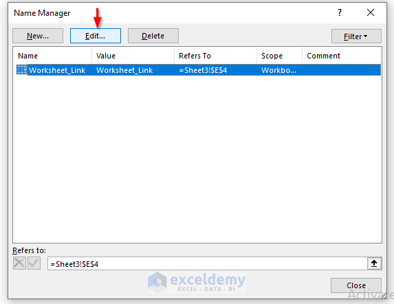
• Select the drop-down list cell, go to Formula, and click on Name Manager.
• Select Worksheet_Link and click Edit.

• In the Refers to field, insert the following formula:

The ADDRESS function is

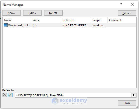
• Click OK.
• The worksheets are linked with the drop-down list.
• We want to go to the Hardware sheet. Select Hardware from the list and click on it.

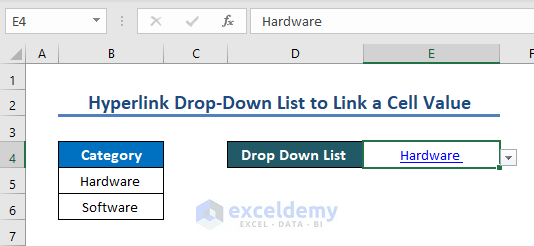
• Excel opens the Hardware sheet.

Read More: How to Create a Drop Down List From Another Sheet in Excel

Things to Remember

⏩ While creating a dynamic drop-down list, make sure that the cell references are absolute (such as $B$4) and not relative (such as B2, or B$2, or $B2)

⏩ In the hyperlink drop-down list, the [abs_num], [a1] are ignored. Put (,,) to do that.

⏩ To avoid errors, check “Ignore Blank” and “In-cell Dropdown”.

Download the Practice Workbook

Related Articles

• Create Excel Drop Down List from Table
• How to Remove Drop Down List in Excel
• How to Create Excel Drop Down List with Color
• How to Create a Drop Down List with Unique Values in Excel
• How to Copy Filter Drop-Down List in Excel
• Excel Drop Down List Not Working

<< Go Back to Excel Drop-Down List | Data Validation in Excel | Learn Excel