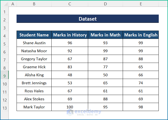
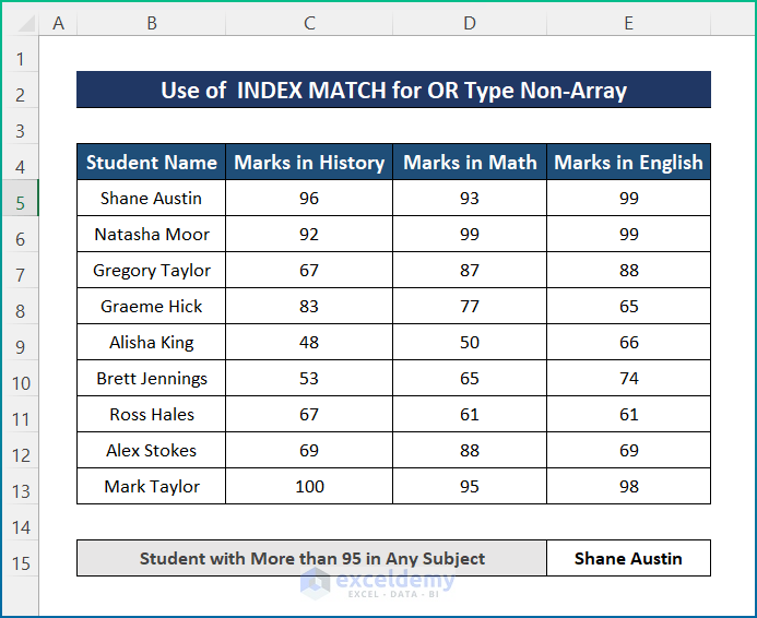
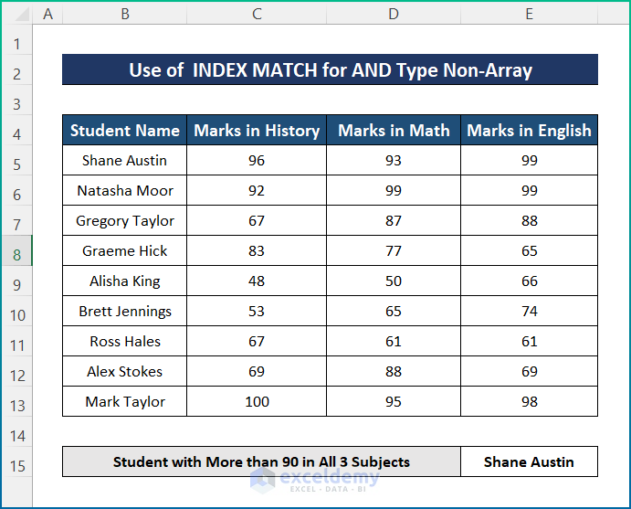
The sample dataset showcases the Annual Examination Record of a school named The Rose Valley Kindergarten, Student Names in column B and their marks in History, Math, and English in columns C, D, and E.
Method 1- Using the INDEX-MATCH function with OR Type Multiple Criteria in Rows and Columns
1.1 INDEX and MATCH Functions with an Array Formula
Steps:
- Select E15 and enter the following formula.
=INDEX(B5:B13,MATCH(TRUE,(((C5:C13)>95)+((D5:D13)>95)+((E5:E13)>95))>0,0))
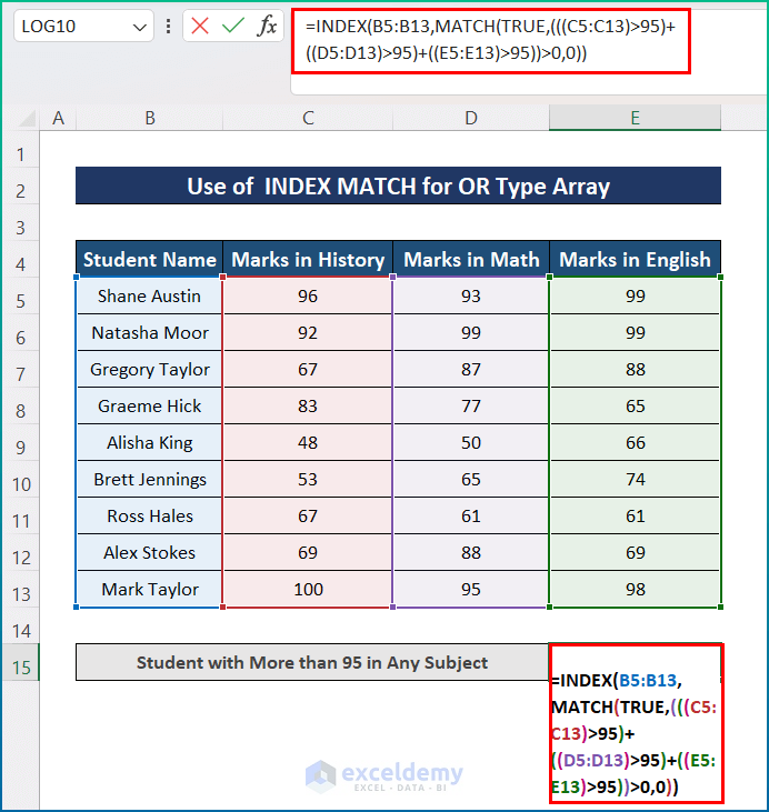
Formula Breakdown:
- With the MATCH function, the 3 criteria: Marks in History, Math, and English are matched with ranges C5:C13, D5:D13, and E5:E13.
- The match type is 1, which gives an exact match.
- The INDEX function gets the name of the student from B5:B13.
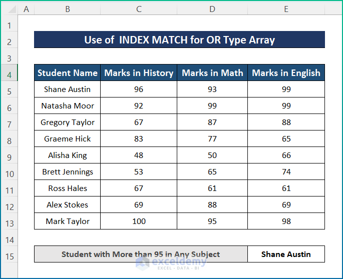
- Press Enter to find the name of the first student with more than 95 in any subject.
1.2 INDEX and MATCH with Non-Array
Steps:
- Select E15 and enter the following formula.
=INDEX(B5:B13,MATCH(TRUE,INDEX((((C5:C13)>95)+((D5:D13)>95)+((E5:E13)>95))>0,0,1),0))
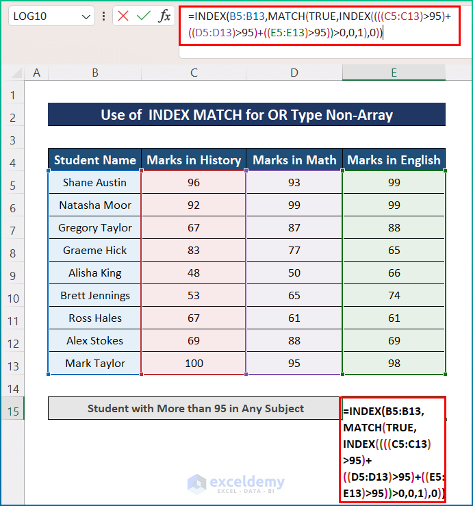
- Press Enter to see the final output.
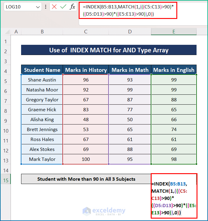
Method 2 – Applying the INDEX-MATCH with AND Type Multiple Criteria in Rows and Columns in Excel
2.1 INDEX and MATCH Functions with anArray
Steps:
- Select E15 and enter the following formula.
=INDEX(B5:B13,MATCH(1,(((C5:C13)>90)*((D5:D13)>90)*((E5:E13)>90)),0))
Formula Breakdown:
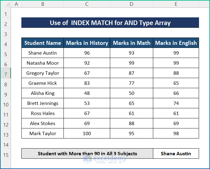
- The MATCH function has 3 criteria: Marks in History, Math, and English are matched with their corresponding ranges, C5:C13, D5:D13, and E5:E13.
- The match is found as 1: an exact match that meets all the conditions.
- The INDEX function provides the name of the student from B5:B13.
- The name of the first student with more than 90 in all 3 subjects will be displayed.
2.2 Using INDEX and MATCH with Non-Array
Steps:
- Select E15 and enter the following formula.
=INDEX(B5:B13,MATCH(1,INDEX((((C5:C13)>90)*((D5:D13)>90)*((E5:E13)>90)),0,1),0))
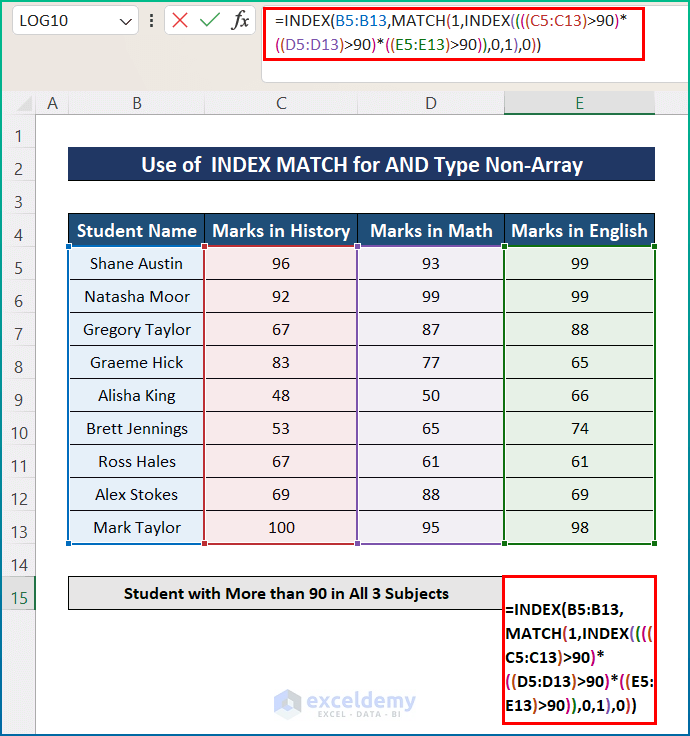
- Press Enter to see the final output.
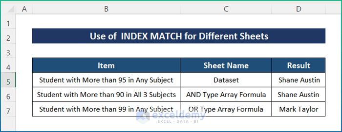
INDEX MATCH for Multiple Criteria in Different Sheets in Excel
Steps:
- Click D4.
- Enter the following formula.
=INDEX(Dataset!B5:B13,MATCH(TRUE,(((Dataset!C5:C13)>95)+((Dataset!D5:D13)>95)+((Dataset!E5:E13)>95))>0,0))
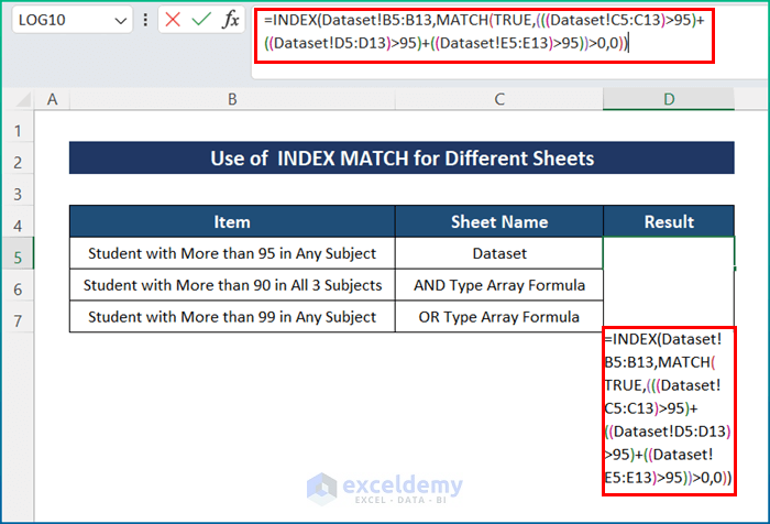
Here, “Dataset” is the name of the sheet from which you want to extract data.
Download Practice Workbook
Download the workbook here.
<< Go Back to Multiple Criteria | INDEX MATCH | Formula List | Learn Excel
Get FREE Advanced Excel Exercises with Solutions!
