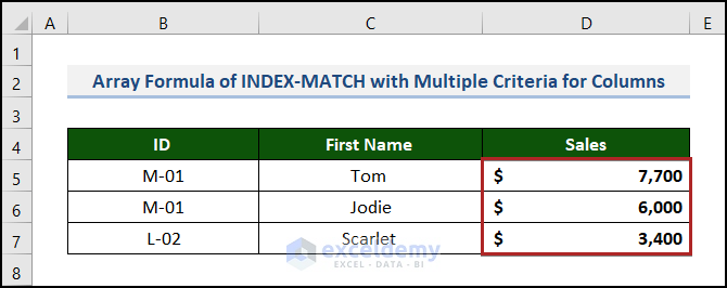
Method 1 – INDEX-MATCH Formula with Multiple Criteria for Columns Only
We’ll use a Monthly Sales Report of a particular organization, containing the ID, First Name, and their respective Sales in columns B, C, and D, respectively.
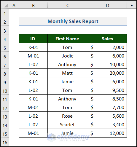
We’ll calculate the Sales amounts of various sales representatives using this worksheet.
Case 1.1 – Using an Array Formula
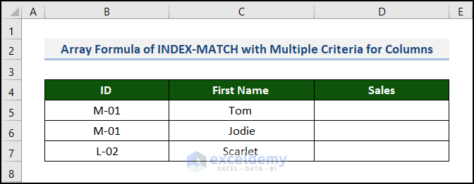
We’ll find Sales for a specific ID and a specific First Name from a different worksheet named “Dataset”.
Steps:
- Make a data range in a new worksheet containing columns ID, First Name, and Sales in the D5:D7 range.
- Name this worksheet Array.
Now we’ll apply the INDEX-MATCH formula to find the Sales amount.
The generic INDEX-MATCH formula with multiple criteria is as follows:
return_range is the range from which the value will be returned.
criteria1, criteria2, … are the conditions to be satisfied.
range1, range2, … are the ranges on which the required criteria should be searched.
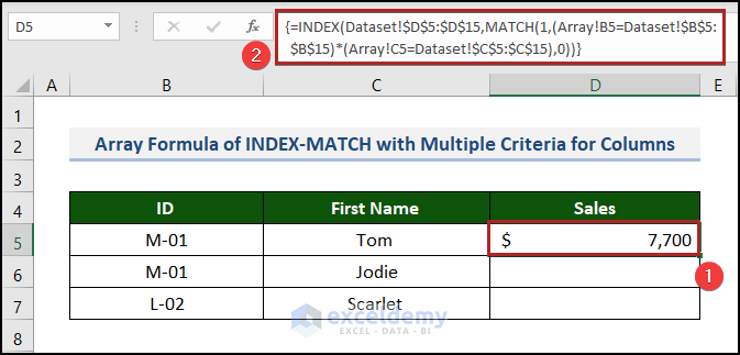
- Select cell D5 and insert the following formula:
=INDEX(Dataset!$D$5:$D$15,MATCH(1,(Array!B5=Dataset!$B$5:$B$15)*(Array!C5=Dataset!$C$5:$C$15),0))
- return_range is Dataset!$D$5:$D$15. Click on the Dataset worksheet and select the data range.
- criteria1 is Array!B5 (M-01).
- criteria2 is Array!C5 (Tom).
- range1 is Dataset!$B$5:$B$15. Click on the Dataset worksheet and select the ID column.
- range2 is Dataset!$C$5:$C$15. Click on the Dataset worksheet and select the First Name column.
- lookup_value for the MATCH function is 1 as it provides the relative location of the row for each of the conditions that are TRUE. The location of the first result is retrieved if there are several instances of 1 in the array.
- match_type is 0.
- Press ENTER.
Note: As this is an array formula, press CTRL + SHIFT + ENTER instead of ENTER if you are using any version other than Excel 365. And don’t put those curly braces around the formula. Excel will automatically add them to the array formula.
- Bring the cursor to the right-bottom corner of cell D5 to activate the Fill Handle tool.
- Double-click on it.
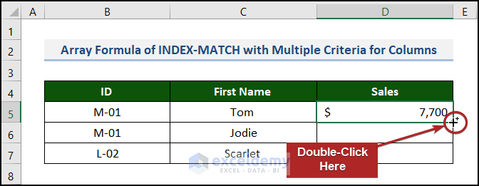
The formula is copied to the cells below.
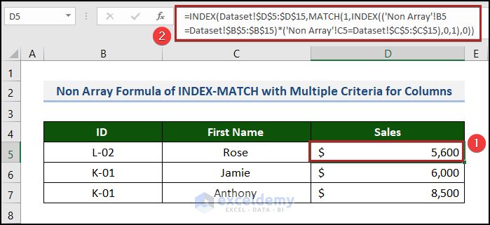
Case 1.2 – Without Using the Array Formula
Steps:
- Make a table like the previous example.
The generic form of the non-array INDEX-MATCH formula is as follows:
- In cell D5, enter the following formula:
=INDEX(Dataset!$D$5:$D$15,MATCH(1,INDEX(('Non Array'!B5=Dataset!$B$5:$B$15)*('Non Array'!C5=Dataset!$C$5:$C$15),0,1),0))
- return_range is Dataset!$D$5:$D$15. Click on the Dataset worksheet and select the data range.
- criteria1 is ‘Non Array’!B5 (L-02).
- criteria2 is ‘Non Array’!C5 (Rose).
- range1 is Dataset!$B$5:$B$15. Click on the Dataset worksheet and select the ID column.
- range2 is Dataset!$C$5:$C$15. Click on the Dataset worksheet and select the First Name column.
- lookup_value for the MATCH function is 1.
- match_type is 0.
- Press ENTER to return the result.
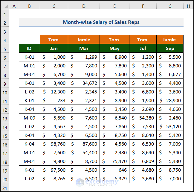
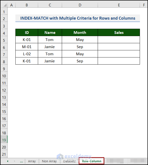
Method 2 – INDEX-MATCH Formula with Multiple Criteria for Rows and Columns
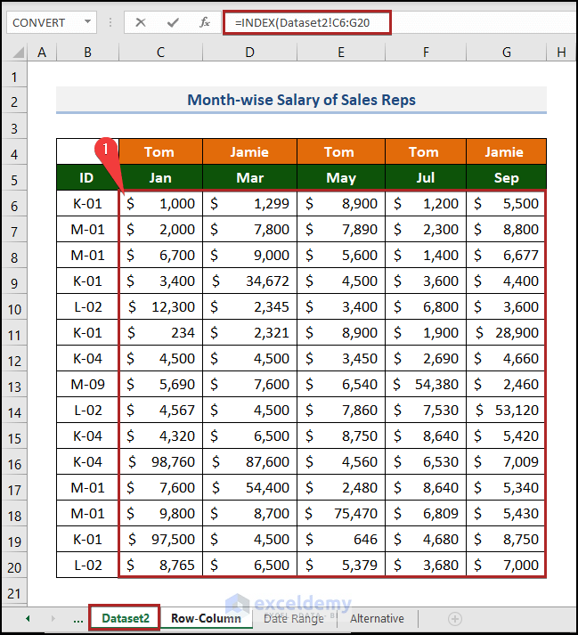
Consider the following dataset where Name and ID of some sales together with Sales of the months Jan, Mar, May, Jul and Sep are given in a worksheet named “Dataset2”.
Let’s find the Sales for some given criteria in a different sheet.
Steps:
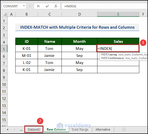
- Construct another table in a different sheet containing the columns Name, ID, and Month where the criteria are given.
- Name this sheet Row-Column.
The format of the INDEX-MATCH formula that we will use is as follows:
- Go to cell E5 and call the INDEX function:
=INDEX(
- Navigate to the “Dataset2” sheet.
- Select the table_array which is the C5:G19 range in the Dataset2 worksheet.
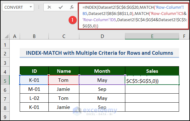
- Complete the full formula as follows:
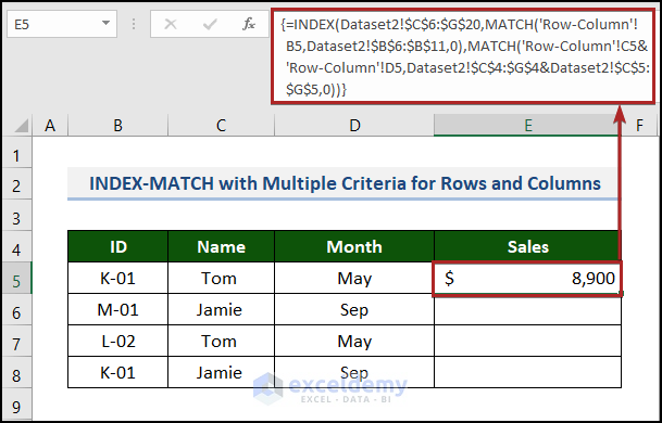
=INDEX(Dataset2!$C$6:$G$20,MATCH('Row-Column'!B5,Dataset2!$B$6:$B$11,0),MATCH('Row-Column'!C5&'Row-Column'!D5,Dataset2!$C$4:$G$4&Dataset2!$C$5:$G$5,0))
- vlookup_value is ‘Row-Column’!B5 (K-01).lookup_column is Dataset2!$B$6:$B$11.
- hlookup_value1 is ‘Row-Column’!C5 (Tom).
- hlookup_value2 is ‘Row-Column’!D5 (May).
- lookup_row1 is Dataset2!$C$4:$G$4.
- lookup_row2 is Dataset2!$C$5:$G$5.
- match_type is 0.
The selected rows and columns are as in the image below.
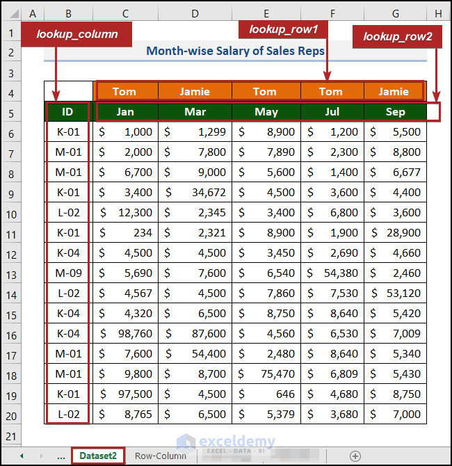
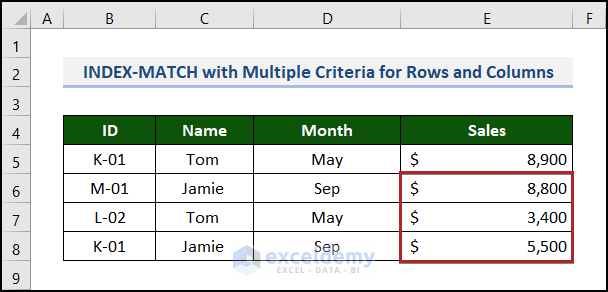
- Press ENTER.
- Use the Fill Handle tool to return results in the lower cells in the column.
How to Apply the INDEX-MATCH Formula with Multiple Criteria for a Date Range
We can extract the price of a certain product on a specific date. We have a list of products with their beginning and ending periods and their corresponding unit price.
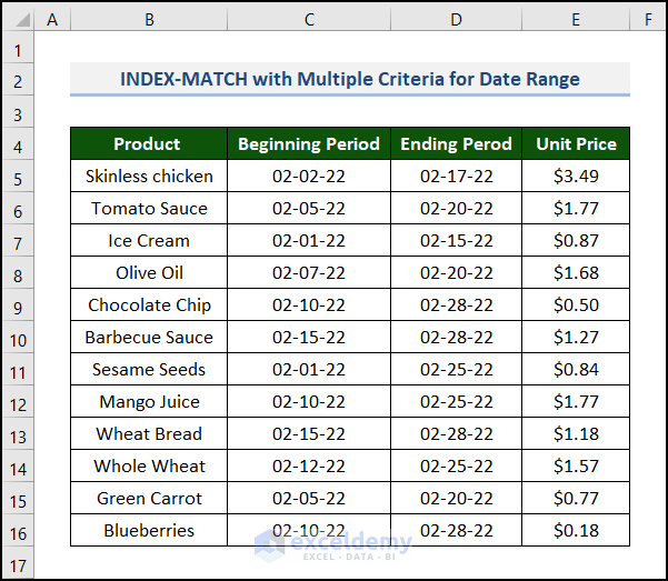
We want to see the price of an Ice Cream on 02-10-22 (month-day-year). If the given date falls within the specified period, we’ll extract the price into a blank cell.
Steps:
- Build an output range in cells D19:D21. We want to find the price for 3 products, but you can customize it according to your needs.
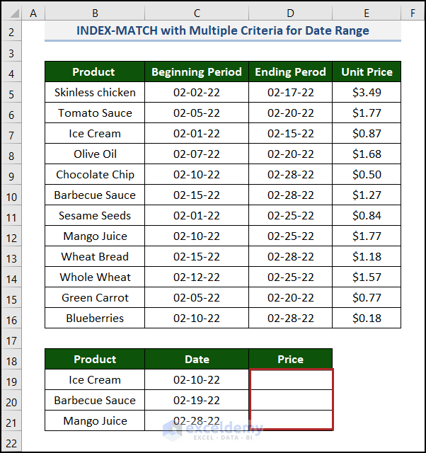
- In cell D19, enter the following array formula:
=INDEX($E$5:$E$16,MATCH(1,(($B$5:$B$16=B19)*($D$5:$D$16>=C19)*($C$5:$C$16<=C19)),0))
- Press ENTER.
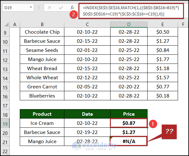
A #N/A error is returned in cell D21 because the date in cell C21 doesn’t lie within the described period in the dataset.
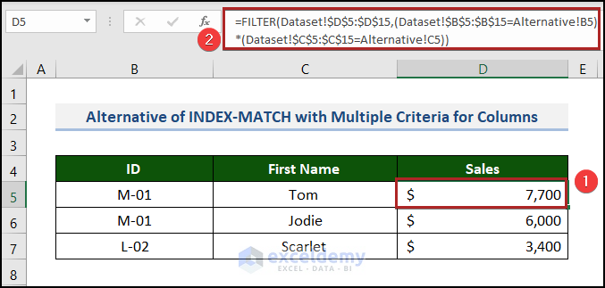
Smart Alternative to INDEX-MATCH with Multiple Criteria
If you are a user of Office 365, you can use the FILTER function.
Steps:
- Create a worksheet like in Method 1.
- In cell D5, enter the following formula:
=FILTER(Dataset!$D$5:$D$15,(Dataset!$B$5:$B$15=Alternative!B5)*(Dataset!$C$5:$C$15=Alternative!C5))
This formula is easier to apply and understand than the previous ones.
- Press ENTER.
Quick Notes
- The INDEX-MATCH is normally an array formula, so press CTRL+SHIFT+ENTER instead of ENTER to get the result.
- If you want to apply the same formula for the rest of the cells, freeze the data range using an absolute cell reference ($). Simply press F4 to apply it to the formula.
Download the Practice Workbook
<< Go Back to Multiple Criteria | INDEX MATCH | Formula List | Learn Excel
Get FREE Advanced Excel Exercises with Solutions!

On step 3 forlmula on pis is like this:
=INDEX(‘Data range’!’Data range’!C5:G19 <<< double "Data range"?
other
array: 'Data range'!$B$5:$B$10 <<< from row 5 to 10 ?
Hi KALI,
Normally when we write down a formula that has references from multiple sheets, the sheet name appears first. That’s why “Data range” appears. You can check the final image of step 3 to get the final formula.
‘Data range’!’Data range’!C5:G19 is corrected now. Thank you for your observation.
‘Data range’!$B$5:$B$10 refers to the range B5:B10. The selected range starts from the 5th row to the 10th row of column B.
Thanks again. Have a good day.