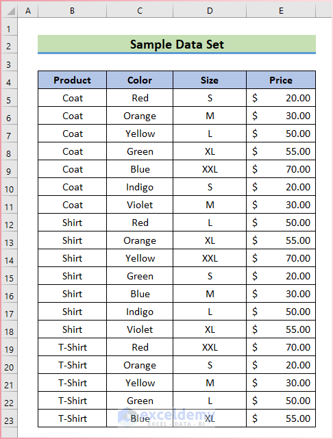
Let’s use the following sample dataset to show how you can use these functions together.
Method 1 – Combine INDEX and MATCH Functions in an Array Formula with Multiple Criteria
Steps:
- Make eight new spaces above the main data set and fill in the first three criteria manually by taking information from the main dataset.
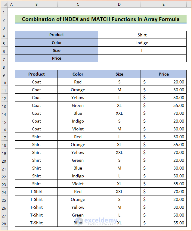
- Insert the following formula in cell D7.
=INDEX(E10:E28,MATCH(1,(D4=B10:B28)*(D5=C10:C28)*(D6=D10:D28),0))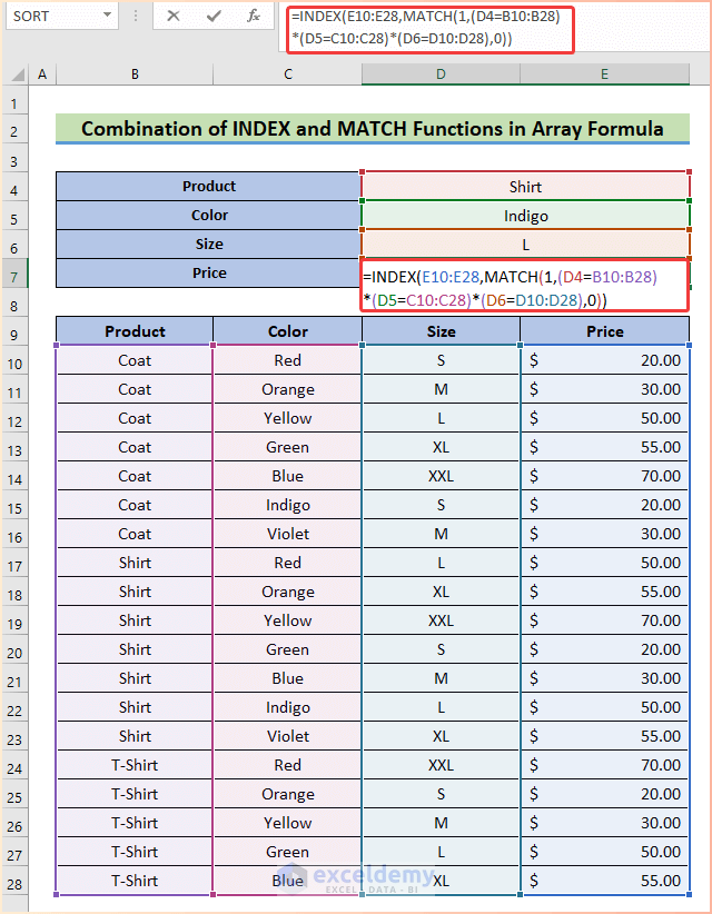
Formula Breakdown
=INDEX(E10:E28,MATCH(1,(D4=B10:B28)*(D5=C10:C28)*(D6=D10:D28),0))
- (B8=B14:B34)*(B9=C14:C34)*(B10=D14:D34): The multiplication operation will search the values to the respective column and return TRUE/FALSE values according to it.
- The multiplication operator (*) converts these values to 0s and 1s and then performs the multiplication operation which converts all other values to 0s except the desired output.
- MATCH(1,(0;0;0;0;0;0;0;0;0;0;0;0;1;0;0;0;0;0;0;0;0),0)): The MATCH function looks for the value 1 in the converted range and returns the position that is 13.
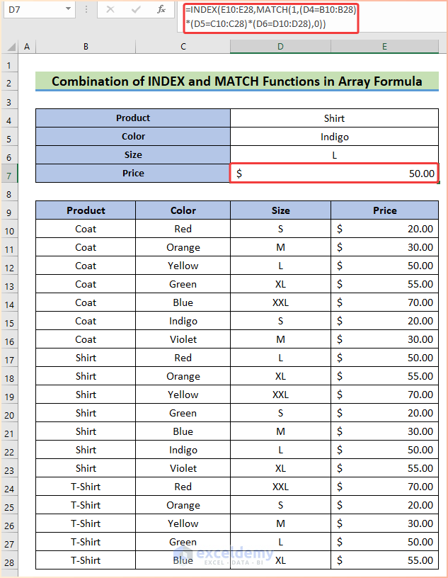
- INDEX(E14:E34,MATCH(1,(B8=B14:B34)*(B9=C14:C34)*(B10=D14:D34),0)): The INDEX function returns the value in the 13th row of the price column which is the desired output that is 50.
- Press Enter and you will see the price of the product that matches the criteria in cells D4, D5, and D6.
Method 2 – Combine INDEX and MATCH Functions in a Non-Array Formula with Multiple Criteria
Steps:
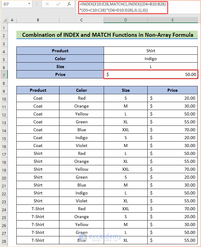
- To find out the price of the product to the given criteria, use the following combination formula in cell D7:
=INDEX(E10:E28,MATCH(1,INDEX((D4=B10:B28)*(D5=C10:C28)*(D6=D10:D28),0,1),0))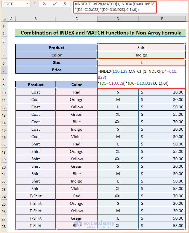
Formula Breakdown:
=INDEX(E10:E28,MATCH(1,INDEX((D4=B10:B28)*(D5=C10:C28)*(D6=D10:D28),0,1),0))
- INDEX((D4=B10:B28)*(D5=C10:C28)*(D6=D10:D28),0,1): The INDEX function will search the values to the respective column and return TRUE/FALSE values according to it.
- The multiplication operator (*) converts these values to 0s and 1s and performs the multiplication operation which converts all other values to 0s except the desired output.
- MATCH(1,INDEX((D4=B10:B28)*(D5=C10:C28)*(D6=D10:D28),0,1),0): The MATCH function looks for the value 1 in the converted range and returns the position that is 13.
- INDEX(E14:E34,MATCH(1,INDEX(B8=B14:B34)*(B9=C14:C34)*(B10=D14:D34),0,1),0)): The INDEX function returns the value in the 13th row of the price column which is the desired output that is 50.
- Press Enter, and you will find the price of the shirt in indigo color and size L.
Method 3 – Combine COUNTIFS, INDEX, and MATCH Functions for Multiple Criteria
Steps:
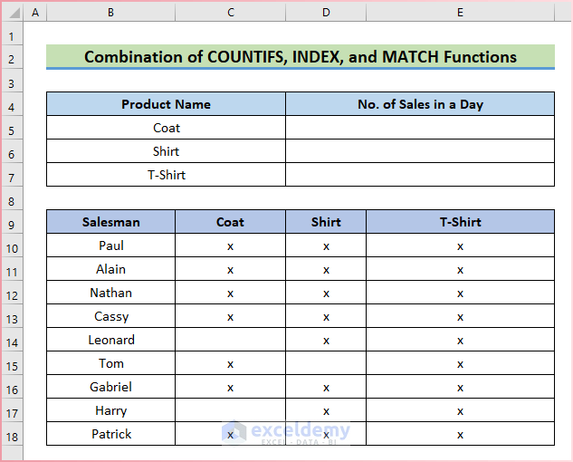
- Input the following data set with the necessary information.
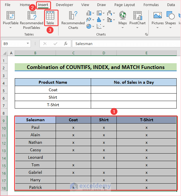
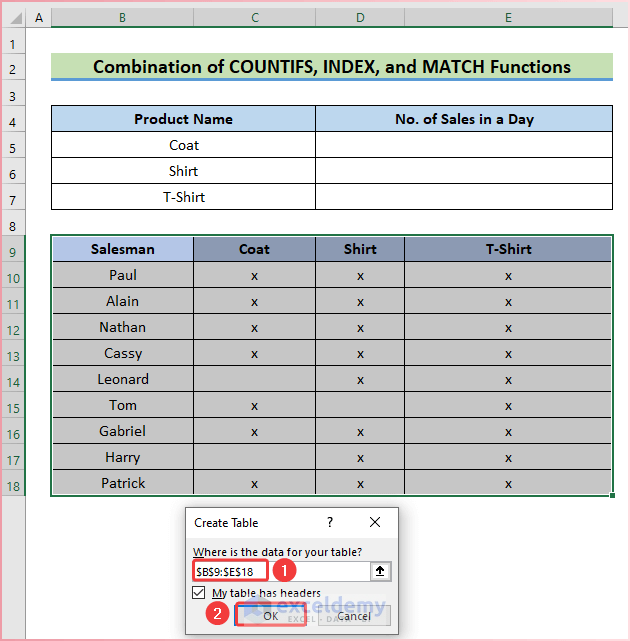
- Select the data range B9:E18 and go to the Insert tab of the ribbon.
- From the Tables group, choose Table.
- In the Create Table dialog box, check the data range and press OK.
- Insert the following combination formula in cell D5 to find out the number of sales of coats in a day:
=COUNTIFS(INDEX(Table4,0,MATCH(B5,Table4[#Headers],0)),"x")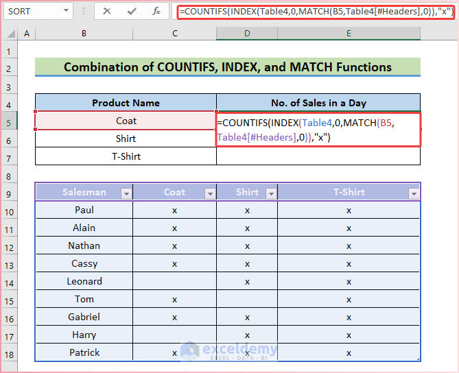
Formula Breakdown
=COUNTIFS(INDEX(Table4,0,MATCH(B5,Table4[#Headers],0)),”x”)
- MATCH(B5,Table4[#Headers],0): The MATCH function uses the cell value of B5 as the lookup value, then the headers in Table4 for the array, and 0 for an exact match.
- INDEX(Table4,0,MATCH(B5,Table4[#Headers],0)): The INDEX function will return the entire column for coat, which is C10:C18 in the above image.
- COUNTIFS(INDEX(Table4,0,MATCH(B5,Table4[#Headers],0)),”x”): The COUNTIFS functions will count cells with “x” in them and will show the total number of cells as the result.
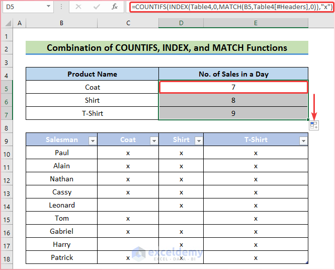
- Press Enter to see the desired value.
- Use AutoFill to get the other results.
Method 4 – Utilize the COUNTIFS Function with Different Logics for Multiple Criteria
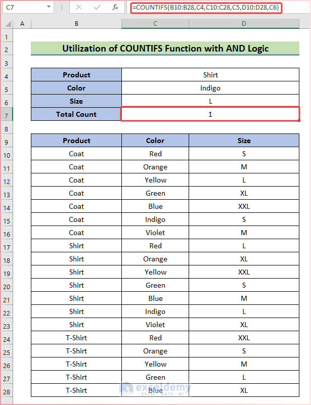
Case 4.1 – COUNTIFS Function with AND Logic
Let’s take the following data set where we want to find out the number of products that match with all the criteria in cell C4, C5, and C6.
Steps:
- Input the following formula in cell C7:
=COUNTIFS(B10:B28,C4,C10:C28,C5,D10:D28,C6)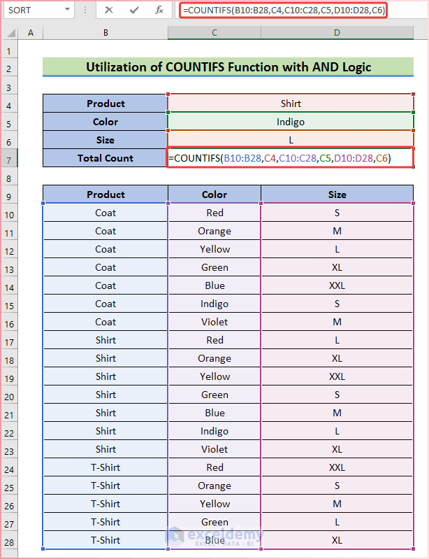
Formula Breakdown
=COUNTIFS(B10:B28,C4,C10:C28,C5,D10:D28,C6)
- COUNTIFS(B10:B28,C4,C10:C28,C5,D10:D28,C6): The COUNTIFS function searches for the values in the respective columns and increases the count if all the criteria are matched.
- There is only one column where all the criteria match. So, 1 is the desired output.
- Hit Enter.
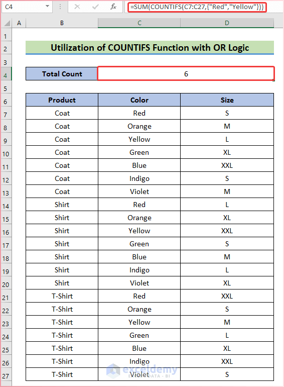
Case 4.2 – COUNTIFS Function with OR Logic
Steps:
- We want to count all the cells that contain yellow and red as cell values.
- Insert the following formula in cell C4.
=SUM(COUNTIFS(C7:C27,{"Red","Yellow"}))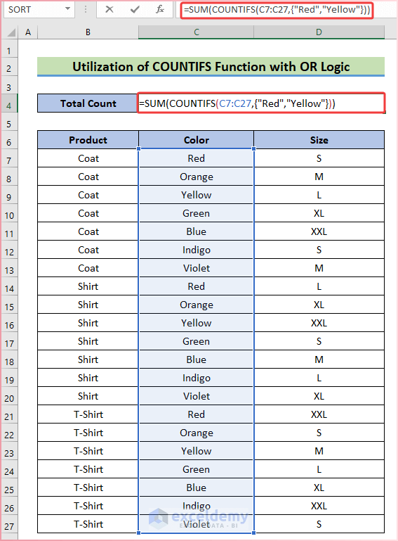
Formula Breakdown
=COUNTIFS(B10:B28,C4,C10:C28,C5,D10:D28,C6)
- COUNTIFS(C7:C27,{“Red”,”Yellow”}): The COUNTIFS function searches for the values in the respective columns and increases the count if any criteria is matched.
- SUM(COUNTIFS(C11:C31,{“Red”,”Yellow”})): As there are three “Red” and three “Yellow” values, the COUNTIF function returns 3,3.
- The SUM function adds the two values and returns the desired output.
- Press Enter.
You can download the free Excel workbook here and practice on your own.
<< Go Back to Multiple Criteria | INDEX MATCH | Formula List | Learn Excel
Get FREE Advanced Excel Exercises with Solutions!

I have utilized Excel for at least a decade. I have ONE Hugh problem with your Excel Seminars. Where where you 10 years ago. Man could I have used your guildance then. You seminars are the best out there – every education and truly a learning experience. Thanks for taking the time and effort – You are a true asset to all.
Dear Seaunders,
Thanks for your appreciation. It means a lot to us.
Regards
ExcelDemy