The Excel file contains information about several sales representatives.
This is an overview.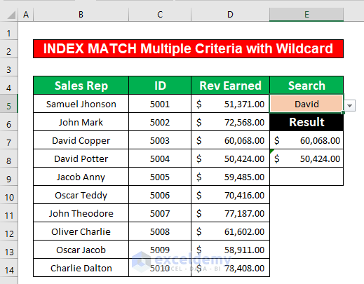
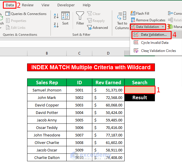
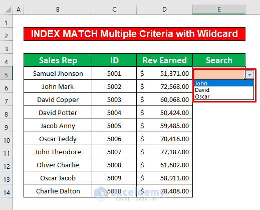
Step 1- Create a Drop Down List to Apply the INDEX MATCH Function with Multiple Criteria and a Wildcard
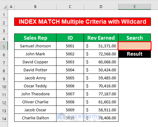
- Select E5.
- In the Data tab, go to
Data → Data Tools → Data Validation → Data Validation
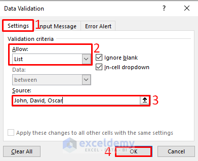
- In the Data Validation dialog box, select Settings.
- Select List in Allow.
- Enter John, David, Oscar in Source.
- Click OK.
- Click OK.
A drop-down list is created.
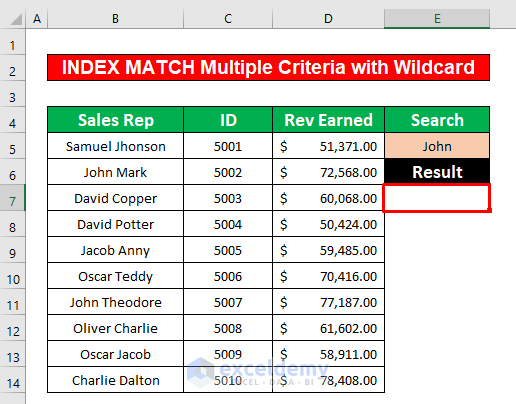
Step 2 – Combine the INDEX and the MATCH Functions for Multiple Criteria using a Wildcard in Excel
- Select E7.
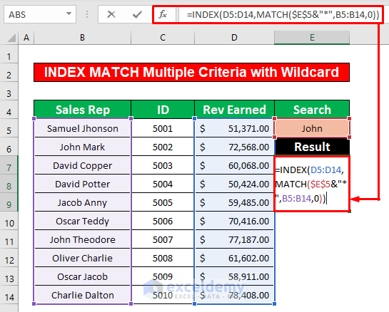
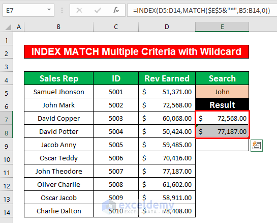
- Enter the INDEX MATCH formula in the Formula bar.
=INDEX(D5:D14,MATCH($E$5&"*",B5:B14,0))Formula Breakdown:
MATCH($E$5&”*”,B5:B14,0)
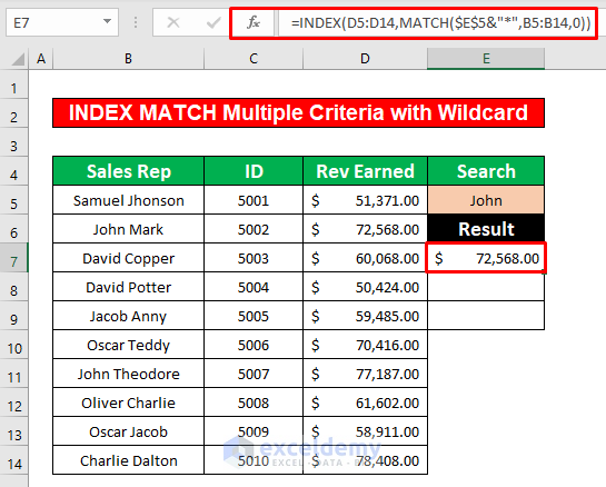
$E$5&”*” is the lookup value; the asterisk is a wildcard character that represents any number of characters starting with John. B5:B14 is the reference range. 0 is used for the exact match. The formula returns 2.
INDEX(D5:D14,MATCH($E$5&”*”,B5:B14,0))
The INDEX function returns $72,568.00: the 2nd row in D5:D14.
- Press ENTER.
You will see the Revenue generated by sales representatives whose name starts with John: $72,568.00.
- Drag down the Fill Handle to see the result in the rest of the cells.
This is the output.
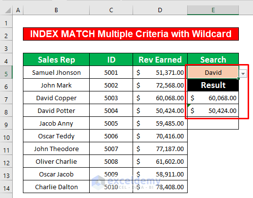
- Change the name in the drop-down list. Check the Revenue generated by sales representatives whose name starts with David:
Download Practice Workbook
Download the practice workbook.
<< Go Back to Multiple Criteria | INDEX MATCH | Formula List | Learn Excel
Get FREE Advanced Excel Exercises with Solutions!

Very clear explanation, but how do I autofill the functions to get the revenue off the others who’s name starts with John or David or whatever? What if there are more people who’s name starts the same? What is the formula in cel E8 for instance.