Excel INDEX MATCH If Cell Contains Text

If the cell contains the text we can use the combination of INDEX & MATCH functions to perform a smart and advanced lookup. It’s a very popular used formula in Excel. In this article, we are going to learn how this two functions combo works with some beautiful explanations and examples.

Introduction to the Excel INDEX Function

Microsoft Excel INDEX function returns the cell value of a defined array or a range.

• Syntax:

=INDEX (array, row_num, [col_num], [area_num])

• Arguments:

array: The cell range or a constant array.

row_num: The row number from the required range or array.

[col_num]: The column number from the required range or array.

[area_num]: The selected reference number of all the ranges that  This is optional.

Introduction to the Excel MATCH Function

Microsoft Excel MATCH function is used to find the position of a lookup value in an array or a range. It returns a numeric value.

• Syntax:

=MATCH(lookup_value, lookup_array, [match_type])

• Arguments:

lookup_value: The searching value in a lookup array or range.

lookup_array: The lookup array or range of cells where we want to search for the value.

[match_type]: This indicates the type of match for the function to perform. There are three types:

An exact match of the value = 0

The largest value which is equal to or less than the search value = 1

The smallest value which is equal to or greater than the search value = -1

Excel INDEX MATCH If Cell Contains Text: 9 Quick Ways

1. Use of INDEX MATCH Functions for a Simple Lookup

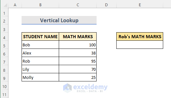
We can use INDEX MATCH functions for a simple column or row lookup in a worksheet. The VLOOKUP function is used only for vertical lookup. So this combo works great here.

1.1 For Vertical Lookup

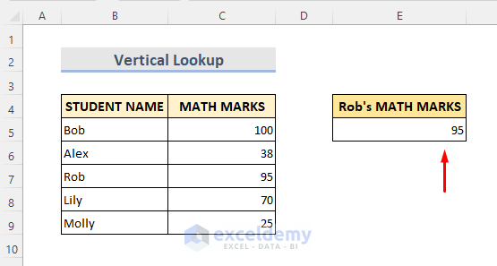
Assuming we have a dataset of student names with their maths marks in vertical position. We are going to look up Rob’s math marks in range B4:C9 and return the value in cell E5.

STEPS:

• First, select Cell E5.
• Next type the formula:

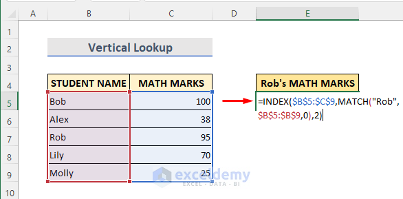
• Now hit Enter for the result.

➥ Formula Breakdown

➤ MATCH(“Rob”,$B$5:$B$9,0)

This will search for the exact match in range B5:B9.

➤ INDEX($B$5:$C$9,MATCH(“Rob”,$B$5:$B$9,0),2)

This will return the value from the range B5:C9.

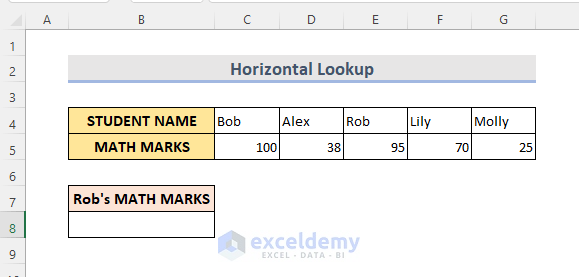
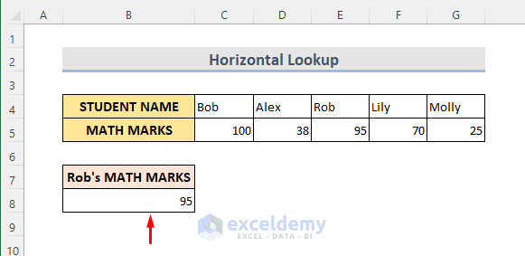
1.2 For Horizontal Lookup

Here we have the same dataset in a horizontal position. We are going to look for Rob’s math marks in range B4:G5 and return the value in cell B8.

STEPS:

• First select Cell B8.
• Now type the formula:

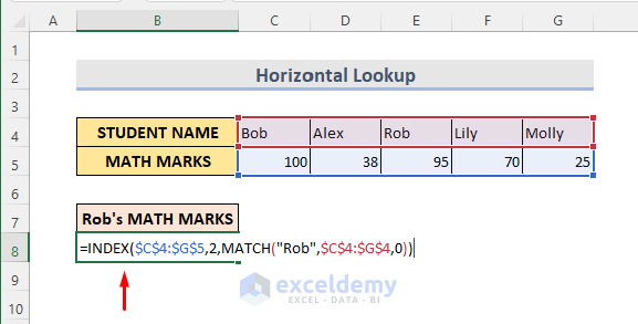
• Finally, press Enter to see the result.

➥ Formula Breakdown

➤ MATCH(“Rob”,$C$4:$G$4,0)

This will search for the exact match in range C4:G4.

➤ INDEX($C$4:$G$5,2,MATCH(“Rob”,$C$4:$G$4,0))

This will return the value from the range C4:G5.

2. Insert INDEX MATCH Function to Lookup Left

To extract the value of the lookup data from its left column, we can use the combination of INDEX MATCH functions. Let’s say we have a dataset (B4:E9) of student names with their English, Maths, Physics marks. We are going to look up Rob’s math marks and return the value in cell G5.

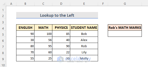
STEPS:

• Select Cell G5.
• Then write down the formula:

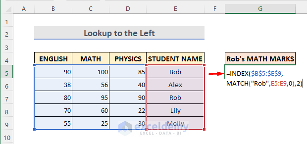
• Hit Enter to get the result.

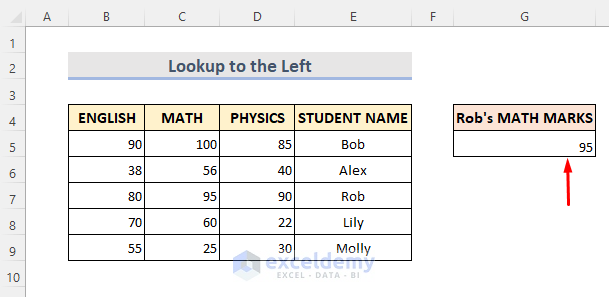
➥ Formula Breakdown

➤ MATCH(“Rob”,E5:E9,0)

This will search for the exact match in range E5:E9.

➤ INDEX($B$5:$E$9,MATCH(“Rob”,E5:E9,0),2)

This will return the value from the range B5:E9.

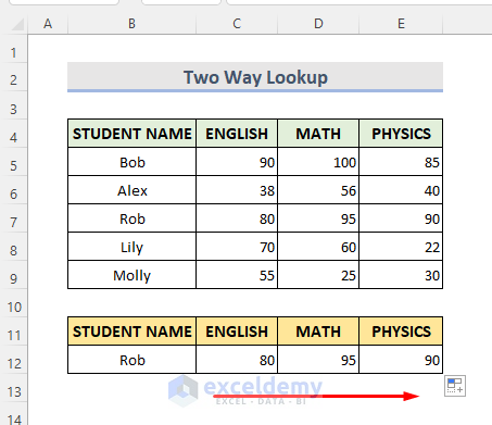
3. Two Way Lookup with INDEX MATCH Functions If Cell Contains a Text

Excel INDEX MATCH functions can beautifully handle the two-way lookup like extracting the values of the lookup data from multiple columns. Here we have a dataset (B4:E9) of different student names with their different subject marks. We are going to extract all the subject marks of Rob in cell C12:E12.

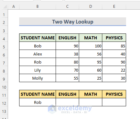
STEPS:

• In the beginning, select Cell C12.
• Now type the formula:

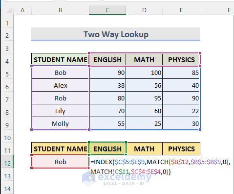
• Press Enter in the end. Use Fill Handle to the right side to autofill the cells.

➥ Formula Breakdown

➤ MATCH($B$12,$B$5:$B$9,0)

This will search for the exact match of Rob in range B5:B9.

➤ MATCH(C$11,$C$4:$E$4,0)

This will search for the exact match of the subject (ENGLISH/MATHS/PHYSICS) in range C4:E4.

➤ INDEX($C$5:$E$9,MATCH($B$12,$B$5:$B$9,0),MATCH(C$11,$C$4:$E$4,0))

This will return the value from the range C5:E9.

4. Use of INDEX MATCH Functions to Lookup Value from Multiple Criteria

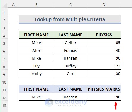
Sometimes we need to combine the lookup values and return their entire information from the defined array. We can use the VLOOKUP function here but it needs a helping column. With the INDEX and MATCH functions combo, we can easily find the value. From the bellow dataset, we want to extract the Physics marks of ‘Mike Hansen’ from the range B4:D9 in cell D12. Let’s follow the instructions below to use the INDEX MATCH functions with Multiple Criteria!

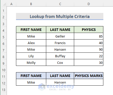
STEPS:

• First, select Cell D12.
• Type the formula:

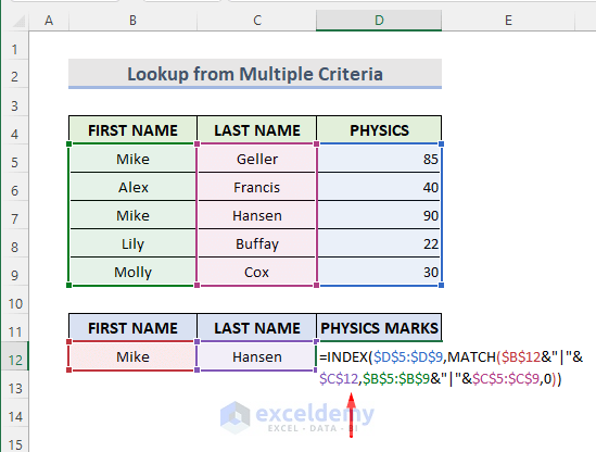
• Finally, hit Enter to see the result.

➥ Formula Breakdown

➤ MATCH($B$12&”|”&$C$12,$B$5:$B$9&”|”&$C$5:$C$9,0)

This will combine the lookup values ‘Mike’ & ‘Hansen’ and search for the exact match in a lookup range $B$5:$B$9&”|”&$C$5:$C$9.

➤ INDEX($D$5:$D$9,MATCH($B$12&”|”&$C$12,$B$5:$B$9&”|”&$C$5:$C$9,0))

This will return the value from the range D5:D9.

5. Use of INDEX, MATCH & SUM Functions to Get Values Based on Text in a Cell

Assume we want to know the total subject marks of the student ‘Rob’. We can use the SUM function along with the INDEX and MATCH functions to get value in cell C12. Let’s follow the instructions below to sum with INDEX-MATCH functions under multiple criteria in Excel!

STEPS:

• Select Cell C12.
• Now write down the formula:

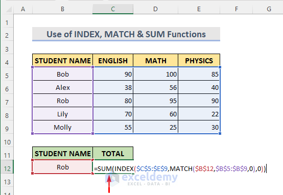
• Then press Enter to see the result.

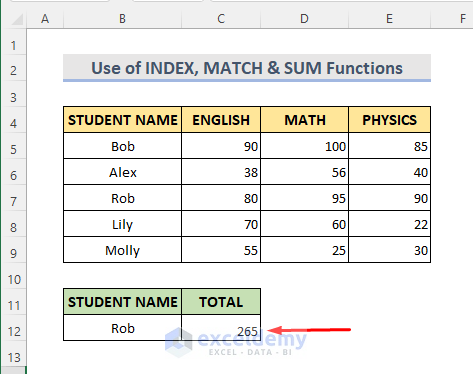
➥ Formula Breakdown

➤ MATCH($B$12,$B$5:$B$9,0)

This will search for the exact match of cell B12 in range B5:B9.

➤ INDEX($C$5:$E$9,MATCH($B$12,$B$5:$B$9,0),0)

This will return the value from the range C5:E9. Here inside the INDEX function, we will input ‘0’ as a column number. This will return all the values in the row.

➤SUM(INDEX($C$5:$E$9,MATCH($B$12,$B$5:$B$9,0),0))

This will sum up all the returned values from the previous step.

6. Insert INDEX MATCH Functions with Asterisk for Partial Match with Cell Text

Asterisk is an Excel Wildcard Character that represents any number of characters in a text string. We use this to look up a value with INDEX MATCH functions if there is a partial match. In the bellow dataset (B4:C9) we have all the students’ full names with their maths marks. Also a dataset with the students’ partial names. We are going to find their math marks and input them in range F5:F9. 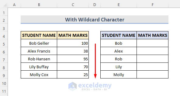Follow the steps below to use INDEX MATCH multiple criteria with wildcard for the partial match of text.

STEPS:

• First, select Cell F5.
• Type the formula:

• Finally, hit Enter and use Fill Handle to autofill the cells.

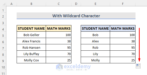
➥ Formula Breakdown

➤ MATCH(E5&”*”,$B$5:$B$9,0)

As a lookup value, we will use E5&”*” as the Asterisk returns with the characters starting with the name ‘Bob’ and any number of the characters after it from the text string range B5:B9.

➤ INDEX($C$5:$C$9,MATCH(E5&”*”,$B$5:$B$9,0),1)

This will return the value from the range C5:C9.

➥NOTE: This formula works if there is only one occurrence of matching. In the case of multiple matching occurrences, it will show only the first matching.

7. Excel INDEX MATCH Functions to Find the Closest Match

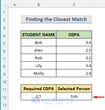
Assume we have a dataset (B4:C9) of students’ CGPA. We are going to find the student who has the closest matched CGPA with the required CGPA in cell C12. Here we will use the INDEX & MATCH functions with the MIN & ABS functions.

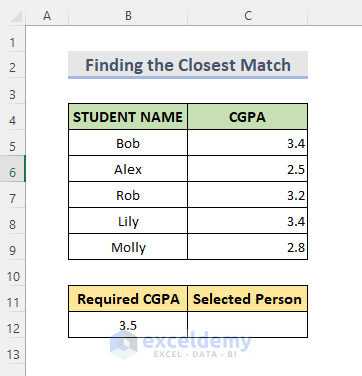
STEPS:

• Select Cell C12.
• Now insert the formula:

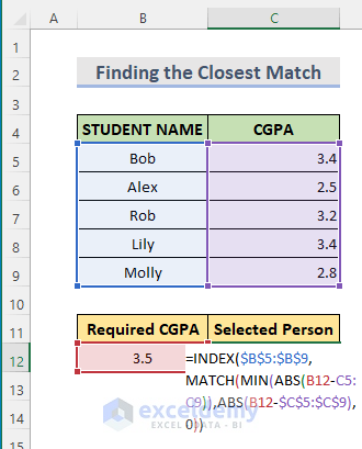
• Next press Enter to see the result.

➥ Formula Breakdown

➤ MATCH(MIN(ABS(B12-C5:C9)),ABS(B12-$C$5:$C$9),0)

This will search for the exact match of cell B12 in range B5:B9.

➤ MIN(ABS(B12-C5:C9)

This will give the minimum difference between the required CGPA and all other CGPA. To make sure the closest (more or less) value, we will use the ABS function here. Inside the MATCH function, the minimum value will be the lookup value.

➤ ABS(B12-$C$5:$C$9)

This will be the lookup array inside the MATCH function.

➤ MATCH(MIN(ABS(B12-C5:C9)),ABS(B12-$C$5:$C$9),0)

Now the MATCH function will find out the position number of the student’s name from the array who has the closest CGPA.

➤ INDEX($B$5:$B$9,MATCH(MIN(ABS(B12-C5:C9)),ABS(B12-$C$5:$C$9),0))

This will return the name of the student.

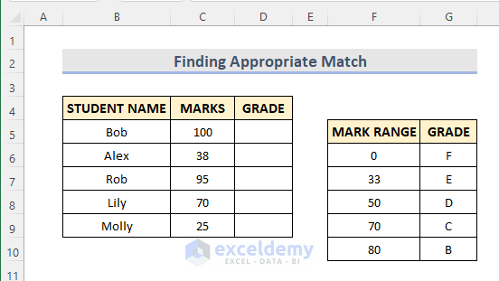
8. Finding Approximate Match with INDEX & MATCH Functions

Here we have a dataset with all the student’s marks. There is also a grading table beside the main table. We are going to find out each student’s grading in range D5:D9 based on the right one (F5:G10).

STEPS:

• First, select Cell D5.
• Next type the formula:

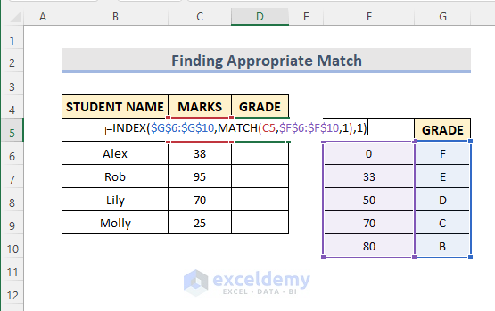
• Finally, press Enter and use Fill Handle to see the total result.

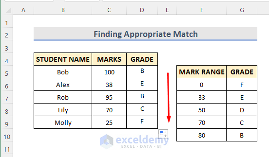
➥ Formula Breakdown

➤ MATCH(C5,$F$6:$F$10,1)

This will search for the exact match of cell C5 in range F6:F10. That means it will go through the marks range and returns the value which will be less than or equal to the lookup value.

➤ INDEX($G$6:$G$10,MATCH(C5,$F$6:$F$10,1),1)

This will return the grade using the position value from the previous step.

9. Case Sensitive Lookup with INDEX & MATCH Functions If Cells Contains a Text

For case-sensitive lookup, a normal lookup won’t work. In this case, Excel INDEX & MATCH functions play an important role. Let’s say we have a dataset of students’ names with their CGPA. There are two students with the same name. The only difference between them is one is written as ‘lily’ and the other one is ‘Lily’. Now we are going to extract Lily’s CGPA and return the value in cell C12.

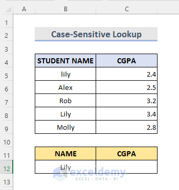
STEPS:

• Select Cell C12.
• Next type the formula:

• Hit Enter to see the result.

➥ Formula Breakdown

➤ EXACT(B12,B5:B9)

This will find the exact match of the lookup value. It will return TRUE for the exact match and FALSE for no match.

➤ MATCH(TRUE,EXACT(B12,B5:B9),0)

This will find the position of TRUE from the previous step.

➤ INDEX($C$5:$C$9,MATCH(TRUE,EXACT(B12,B5:B9),0),1)

This will return the CGPA using the position value from the previous step.

Practice Workbook

Download the following workbook and exercise.

Conclusion

If the cell contains text, we can easily combine Excel INDEX & MATCH functions to look up the value. There is a practice workbook added. Go ahead and give it a try. Feel free to ask anything or suggest any new methods.

<< Go Back to Multiple Criteria | INDEX MATCH | Formula List | Learn Excel