Latest Posts From Saquib Ahmad Shuvo

This is an overview: Download Practice Workbook Download the practice workbook. Spell Check.xlsm 1. Using the Spelling Command to ...
Download Practice Workbook Fonts in Excel.xlsx Method 1 - Using the Excel Ribbon Options Select the cell containing the text you want to ...
This is an overview. Download Practice Workbook Download the practice workbook. Checkbox in Excel.xlsm How to Add a Checkbox in ...

In this article, we will demonstrate the use of the SUMIF function with date range in Excel. In this section, we will look at how to use the SUMIF function ...

In this article, we will demonstrate how to create a dynamic range in Excel. We will go over topics including defining dynamic ranges, using dynamic range ...
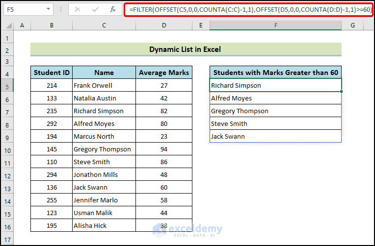
Download Practice Workbook Dynamic List.xlsx Method 1 - Using FILTER and OFFSET Functions Based on Single Criteria: We will combine FILTER ...
Here are some cases of Excel not filtering the entire column. Excel Not Filtering Entire Column: 9 Possible Reasons with Solutions Reason 1 - ...

Method 1 - Insert Single Row with Values Use an Excel VBA code to insert a single row with values into a dataset that contains student names and grades. ...

There are various ways to display messages for 5 seconds using VBA in Excel. In the video below, we use VBA code to display a MsgBox for five seconds before ...

If you are looking for some special tricks to know how to use OFFSET for cell reference in Excel, you've come to the right place. We’ll show 5 suitable methods ...

If you are looking for some special tricks to know how to use the DOLLAR function in Excel, you've come to the right place. We’ll show 5 suitable examples to ...

Example 1 - Calculate the Sales Bonus We have two columns containing Sales Target and Sales Achieved for some products. We’ll check in Column E if the ...

If you are looking for some special tricks to know how to create a progress thermometer in Excel, you've come to the right place. There is one way to create a ...
We'll use the dataset below, which includes student names and corresponding grades. We will scale the data in the Marks column. Method 1 - ...

Step 1 - Prepare the Work Plan Timeline Enter the data Headlines. Enter the Project name and the tasks. Enter the names of the workers responsible ...
- 1
- 2
- 3
- …
- 9
- Next Page »
See Our Reviews at


1. First, use the now() function to extract time from the date in another column: copy the date, press Ctrl+1, select Custom, and then enter h:mm AM/PM in the Type field. To copy the date you have to use the formula:
= cell reference
2. After getting the Time column, you need to use the IF function to find the Present and Late column. The formula will be:
=IF(Time column cell>$absolute reference cell,”Present”,”Late”)
In this case, 7:30 AM would be the absolute cell reference.
3. In order to find only the Late comers, you need to use the IF function. The formula will be
=IF(Present and Late column cell=$absolute reference cell,”Late”, “”)
4. Using Pivot Table, you can transfer the Present and Late Column to another sheet. Select the Insert tab, select Pivot Table, enter the whole table in the range option and finally select New Worksheet. You must select the rows or columns that you want to display in the pivot table after the PivotTable Fileds pane appears.
Thank you so much for sharing this information with me.
It is effective. Thank you for providing this information.
Hi MICHELLE,
Greetings and thank you for your inquiry.
To apply the above formula to the extra payment, you need to change the formula in cell H12 as follows:
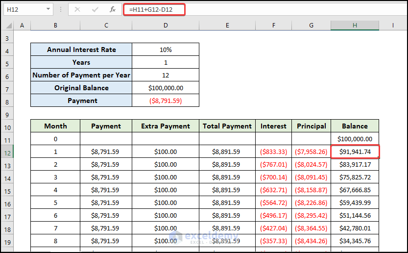
=H11+G12-D12
This means (Original Balance-Principal-Extra Payment).
Greetings, WALKER!
Your question is greatly appreciated.
The process is the same if you have different country codes. Just change the country code number. For instance, if you want to change a telephone number to a UK format.
Firstly, select the phone numbers from the range of cells. Next, press Ctrl+1. Select Custom from the Format Cells dialog box, then type +44 (000) 000-0000. Click on OK.
Greetings, Huda.
I appreciate you asking this question. Solved examples are available about distribution or transportation problems. You can find it here “Solving Transportation or Distribution Problems using Excel Solver”.
Greetings, IVAN
I appreciate your question. This article explains how to save multiple Excel sheets to CSV. We demonstrate not only the VBA method but also two very effective methods: using Google Sheets and using an online converter. Here, we also illustrate some basic methods to save multiple sheets of Excel to CSV by using Save As command, ‘CSV UTF-8′ Format, and CSV UTF-16 Encoding Option.
Greetings ALAN,
I appreciate you asking this question. Excel will automatically generate this date in the intermediate stage when you are trying to create a gannt chart. During the Final stage, you will notice that project-1’s starting date has been corrected.
Hello Marcel,
Greetings. I could not understand your question. It would be much easier for me to answer your question if you could send me your Excel workbook at [email protected].
Dear Macel,
Greetings. In order to track project progress in Excel and incorporate additional tasks, milestones, and percentages, you can follow these steps:
Open your project tracker in Excel or create a new one.
Make sure your tracker has the necessary columns to accommodate the new tasks. You can add columns for line numbers, X-ray, hydrotesting, painting, NDT (non-destructive testing), dye penetration, and any other relevant tasks you mentioned.
To maintain the formatting and calculations in your existing tracker, insert new rows for the additional tasks. Right-click on the row number where you want to add the new tasks and select “Insert” from the context menu.
Enter the task names and other relevant details in the newly inserted rows.
Adjust any formulas or calculations in your tracker to include the new tasks. For example, if you have a column for task completion percentages, you may need to update the formulas to include the newly added tasks in the calculation.
To ensure that the total progress always adds up to 100%, you can either manually adjust the percentages or create formulas that automatically calculate the percentages based on the completed tasks.
To add milestones to your tracker, you can designate specific rows as milestone markers. You can either create a separate column for milestones or use conditional formatting to visually highlight the milestones. You can also add a separate column to describe each milestone and provide additional details if necessary.
Remember, the specific steps may vary based on your Excel version and the structure of your project tracker. Experiment with different approaches to find the one that suits your needs best.
Dear Macel,
In the comment above, I already answered your question.
Dear Macel,
In the comment above, I already answered your question.
Dear Marcel,
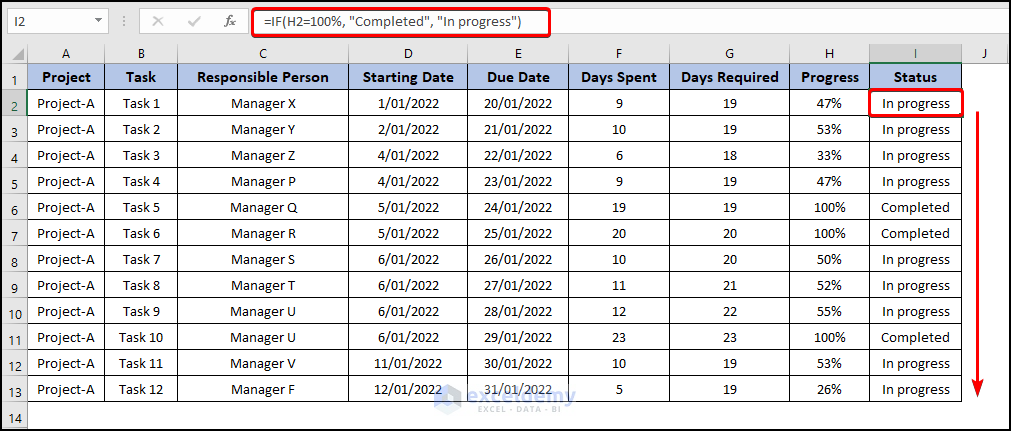
Apply the following formula in the Task status column, then drag it down to alter the task status dynamically.
=IF(H2=100%, “Completed”, “In progress”)
Dear Macel,
Greetings. When tracking project progress in Excel, it is important to provide your boss with concise and relevant information. Here are some recommendations to address your questions:
Daily Project Report: When sending a daily project report to your boss, focus on key updates and highlights. Include information such as completed tasks, milestones achieved, any critical issues or risks, and a summary of overall project progress. It’s not necessary to send the entire project tracker every day; instead, provide a brief overview or summary.
Task Status and Overall Project Completion: If you manually add an extra day to your overall project completion tracker without updating the task status, the completion status will remain unchanged. Task status should reflect the progress of individual tasks, while the overall project completion tracker represents the aggregate progress. To ensure accurate reporting, make sure to update both the task status and the overall project completion tracker accordingly.
Apply the following formula in the Task status column, then drag it down to alter the task status dynamically.
=IF(H2=100%, “Completed”, “In progress”)
Dear EMMA PALMER,
Greetings. Thank you for your question. I have provided a primary solution to your question. It would be much easier for me to solve your problem if you could send me your dataset and Excel workbook.
Yes, it is feasible to use both of the formulas you gave. However, your usage of syntax is not totally accurate. The proper syntax for each formula is as follows:
Formula 1:
=IF(COUNTIFS(R2,”value1*”,S2,”status1″),”aaa”,”bbb”)
This formula checks if the value in cell R2 starts with “value1” and the value in cell S2 is “status1”. If both conditions are true, it returns “aaa”; otherwise, it returns “bbb”.
Formula 2:
=IF(OR(COUNTIF(R2,”value1*”), COUNTIF(R2,”value2*”)), “aaa”, “bbb”)
This formula checks if the value in cell R2 starts with either “value1” or “value2”. If either condition is true, it returns “aaa”; otherwise, it returns “bbb”.
Dear CHRIS B.
Greetings. Thank you for your inquiry. I am not quite sure in which step you get the first error. You might be experiencing that issue as a result of improper code application.
Hello RICK,
Greetings. Your interpretation is accurate.
Dear JENNI,
Greetings.
According to what I know, there isn’t a way to combine the modules in Excel VBA so that they both function and you can choose multiple items from each column.
The task of selecting multiple items from a data validation drop-down list can be accomplished using the VBA code below.
Dear JENNI,
Greetings. I would appreciate it if you could send me your Excel workbook so that I can solve your issue quickly.
Hello CASSIE,
Greetings. Use Excel VBA to quickly complete your task. In Excel VBA, you can use the following code to only copy the cells in columns A through J (inclusive) rather than the entire row:
The End(xlUp) method, which locates the final non-empty cell in the column, is used in this code to obtain the last row in column A first. Then, using the Range object and Copy method, it copies the data from columns A to J.
This code can be changed if you want to perform additional operations on the copied data or paste it in a different place.
Hello SAZ,
Greetings. Using Excel formulas and charts, you can display the percentage of each course that has been completed for each team and the entire organization. The steps are as follows:
1) Calculate the percentage completed for each course for each person:
You can use a formula to count the number of completed courses and divide it by the total number of courses for each person. For example, if the number of courses is in column B and the completed courses are in column C, the formula in column D could be:
=IFERROR(C2/B2,0)
Calculate the percentage completed for each course for each team:
2) You can use the AVERAGEIF function to calculate the average percentage completed for each course for each team. For example, if the team name is in column A and the percentage completed is in column D, the formula in column E could be:
=IFERROR(AVERAGEIF(A:A,A2,D:D),0)
Calculate the percentage completed for each course for the organization as a whole:
You can use the same AVERAGEIF function to calculate the average percentage completed for each course for the entire organization. For example, if the percentage completed is in column D, the formula in column E could be:
=IFERROR(AVERAGEIF(D:D,”>0″),0)
Create a chart:
3) You can create a column chart to visualize the percentage completed for each course for each team and for the organization as a whole. Select the data range that includes the course names and the percentage completed columns, then go to Insert > Charts > Column Chart and choose the type of chart you prefer. You can also add labels, titles, and legends to the chart as needed.
With the help of these steps, you ought to be able to monitor the percentage of each course that has been completed by each team and the organization as a whole.
Dear Deezballs,
Greetings. Usually, it refers to having three sets of data that you want to plot on the same graph when making a line graph in Excel with three variables. In general, using three variables when making a line graph in Excel means you want to see how three different sets of data relate to one another over time or across a range of values.
Hello NIK ABDUL AZIZ,
Greetings. Use the following code in Excel VBA to insert entire rows beneath a number entry in a cell.
The Worksheet_Change event can be used to automate the aforementioned code so that it is not visible to the user. Anytime a cell in the worksheet is modified, this event will be triggered.
Hello JORDAN,
Greetings. You can easily change the color of the fill based on the project by following the steps below.
First, double-click on the particular task of the specific project in the Gantt chart. Therefore, the Format Data Point window will appear. Next, in the Format Data Point, you have to select Fill & Line and then choose Solid Fill. Then, you have to enter your required color for the data point. You have to follow the same procedure for the other tasks in the specific project. You can alter the fill’s color in accordance with the project in this way.
The steps listed below must be followed if you want to instantly change the Gantt chart’s color.
First, click on the task of any project in the Gantt chart. Therefore, the Format Data Series window will appear. Next, in the Format Data Series, you have to select Fill & Line and then choose Solid Fill. Then, you have to enter your required color for the Data series. Based on the color you enter, this process will create a similar color for the entire Gantt chart.
Hello NIK AZIZ,
Greetings. I didn’t understand your query; could you kindly write it down in detail so that I can give you the required answer?
Hi WOLFIXX,
Greetings. Thanks for commenting. You just need to select Administrative Templates from User Configuration from the Local Group Policy Editor dialog box.
Hi MR STEVEN J BUNTING,
Greetings. Thanks for commenting. Yes, you can count cells by color with conditional formatting in Excel. To do this, you can follow three procedures: filter feature, table feature, and sort feature. Please follow the following articles if you would like to know more details.
Count Cells by Color with Conditional Formatting in Excel (3 Methods)
Hi Carrie,
Greetings. Thanks for commenting. Yes, you can change the color scheme by following the below process.
Select the data range where you want to apply Conditional Formatting. Then click as follows: Home > Conditional Formatting > Highlight Cells Rules > Equal To.
Soon after, a Conditional Formatting dialog box named Equal To will open up
Type the name of the Region for what you are looking for duplicates.
Then click on the drop-down icon from the right side of the dialog box and select Custom Format.
Therefore, the Format Cells window will appear, and select the Fill option. Then choose your desired color.
Finally, just press OK
Greetings. Thank you for your question. If any of the above steps aren’t working, try searching for Microsoft Office updates and staying up-to-date with the software, or install Microsoft 365. Sometimes the little bugs and irregularities get eliminated by new updates. Then again, if you are up to date with the updates, then it might be time for a clean reinstallation of the software. By installing the updated version, you can solve the problem. To install the updated version, you have to follow the following process:
Firstly, in Excel, you have to open File > Account.
Next, select Update Options, and click on Update Now.
Greetings. You must carry out the subsequent steps if you want to resolve the issue.
When you run the VBA code, you will find a Microsoft Excel prompt box asking you to enter the first date.
Subsequently, enter the date that you want to insert in the first worksheet. Enter it using the DATE function in Excel.
To fix your problem, you have to enter the formula:
=DATE(2022,12,28)
Year, month, and day are shown, respectively, as (2022,12,28).
Next, click on OK.
Now, another Microsoft Excel prompt box will appear that will ask you to enter the increment.
Enter the increment, and then click on the OK button.
Thank you for your question. To solve the problem, you have to follow the process and code below.
1) Firstly, write down the VBA code below.
2) By running the code, a “File Open” window will appear on your computer.
After that, click on the workbook you want to collect data from.
Then, click on the OK button.
3) Then, select the data from the source file by dragging over the range, and then click OK.
4) After selecting the data range. Now select the destination range where you want to put the data.
And, click OK.
5) In the end, this will close the source file and the data will copy on the destination file.
Below is a link to an article where you will find three different methods and different types of VBA codes that will resolve your issue.
https://www.exceldemy.com/excel-vba-copy-data-from-another-workbook-without-opening/
Thank you for your question. Yes, you can prepare it on an empty Excel sheet so that it will balance automatically when the figure is entered.
Thank you for your question. This article already demonstrates the solution. To exercise while you read this article, you can download the practice workbook from the Download Practice Workbook section.
Hello HUYNH LE TUAN,
Thank you for your question. I couldn’t understand your question properly. Could you please provide your Excel workbook? It would be easy for me to solve the code error if you send me a copy of your Excel workbook. You can send your workbook here- [email protected]
Hi JOHN,
It is a pleasure to hear that this article has been helpful to you.
Hi GENOBLE,
Your question is greatly appreciated. You can easily fix your error by enabling Excel’s GetPivot Data function. If you want to enable Excel to use the GETPIVOTDATA function when you point to pivot table cells at the time of creating a formula, choose PivotTable Tools ➪ Analyze ➪ PivotTable ➪ Options ➪ Generate GetPivot Data command. Now, you can easily reference a cell on another tab in the main pivot cell.
Hi Murtaza,
Your question is greatly appreciated. By following the article “How to Update Links Without Opening File in Excel”, you can easily fix your report so that you don’t have to open multiple files.
Greetings, LOIACONO.
I appreciate you asking this question. You have to follow the “3 Shop Scheduling Problem” example from this article. If you wish to do the calculation at a time/hour level instead of a day level, you need to input hours instead of days in the Days needed column. You must then follow the example’s rest of the process to arrange jobs in a way that maximizes machine utilization.
Greetings, ALF.
It was helpful to receive the information you provided.
Greetings, Raja.
I appreciate you asking this question. You can find it here “Sequencing problem using Johnson’s algorithm of scheduling n-jobs on 2-machines”
Hi Peter,
Thank you.