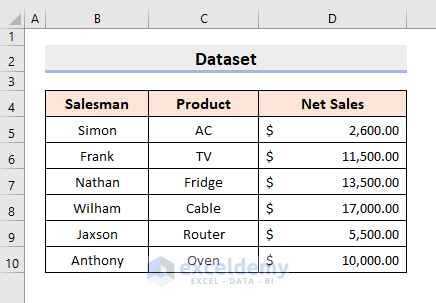
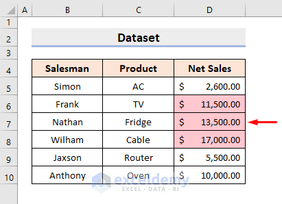
The sample dataset contains the Salesman, Product, and Net Sales of a company.
The Conditional Formatting feature in Excel is used to format the font color, border, etc. of a cell, based on a given condition.
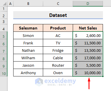
In this case, we will color the sales in Light Red where it exceeds $10,000.
STEPS:
- Select the range of cells to work with.
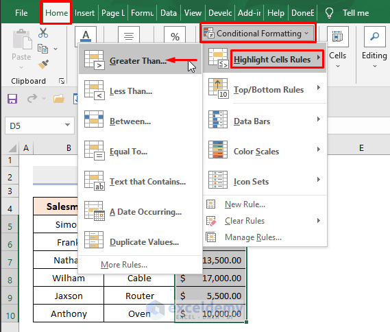
- Select Greater Than from Highlight Cell Rules options in the Conditional Formatting drop-down list under the Home tab.
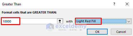
- A dialog box will appear. Type 10000 in the Format cells that are GREATER THAN box and select Light Red Fill in the with section.
- Press OK.
- Sales which exceed $10,000 appear in light red color as in the following picture.
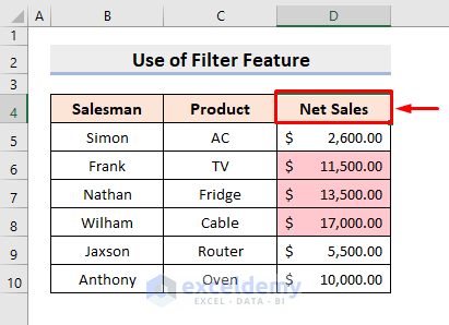
Method 1 – Applying Excel Filter to Count Cells by Color with Conditional Formatting
STEPS:
- Select cell D4.
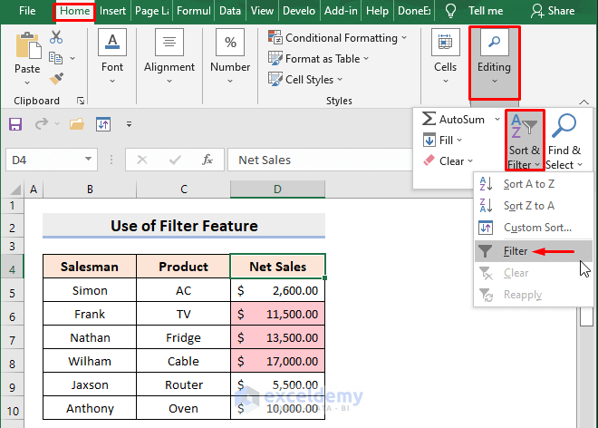
- Under the Home tab, in the Editing group, select Filter from the ‘Sort & Filter’ drop-down.
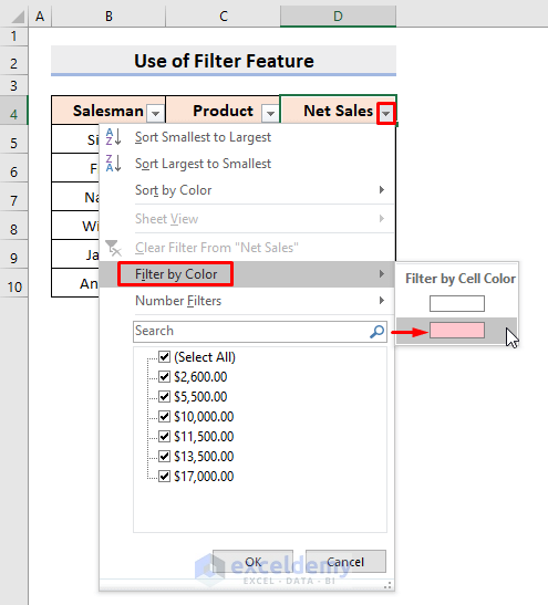
- Select the drop-down symbol beside the header Net Sales.
- Select the light red color from the Filter by Cell Color options as shown below.
- Select cell D12 and type the formula:
=SUBTOTAL(2,D6:D8)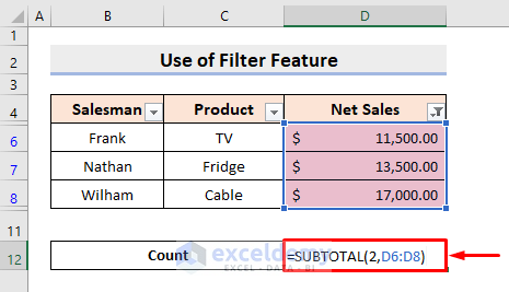
Here, 2 is the function number for counting and D6:D8 is the range.
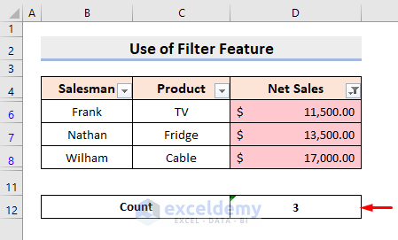
- Press Enter and you’ll get the desired count result.
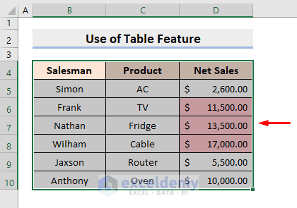
Method 2 – Counting Colored Cells with Conditional Formatting with Excel Table
STEPS:
- Select the range.
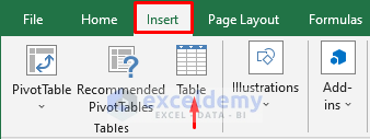
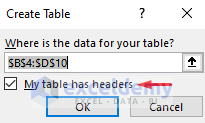
- Under the Insert tab, select Table.
- A dialog box will pop up. Click the My table has headers box.
- Press OK.
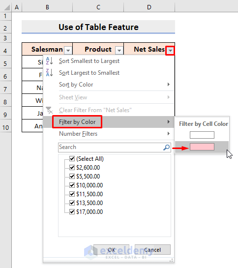
- Click the drop-down symbol beside the header Net Sales.
- Select the light red color from the Filter by Cell Color options in the Filter by Color list.
- This will return the table with the selected cell color only.
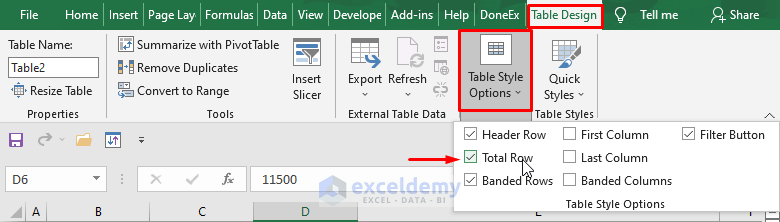
- Select any cell inside the table and you’ll see a new tab named Table Design.
- Check the Total Row box which you’ll find in the Table Style Options list under the Table Design tab.
- A new row just under the table will appear with the sum of the sales in cell D11.
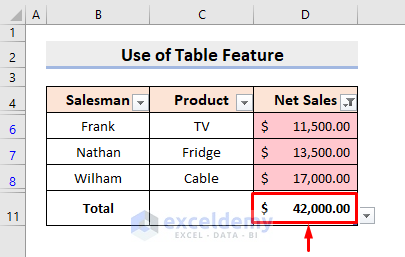
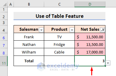
- Click the drop-down symbol in cell D11 and select Count from the list.
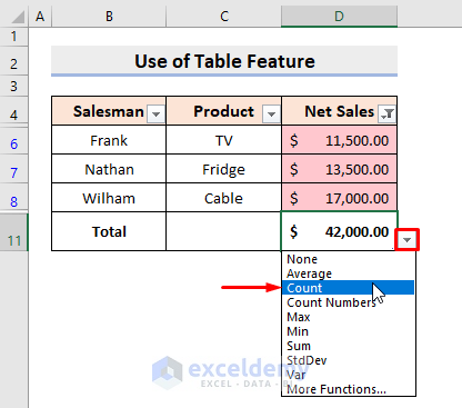
- Cell D11 will show the colored cell count.
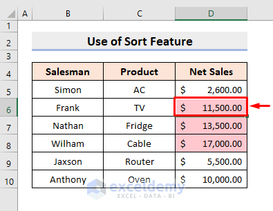
Method 3 – Using Excel Sort Tool to Count Conditionally Formatted Colored Cells
STEPS:
- Select any colored cell you want to work with. In this case, cell D6 is selected.
- Right-click on the mouse and select Put Selected Cell Color On Top from the Sort option.
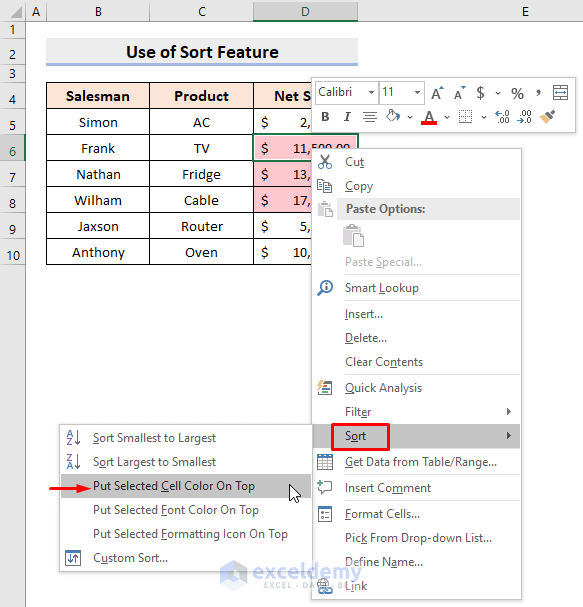
- Select the colored cells as shown below.
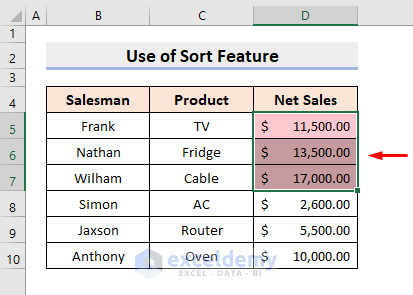
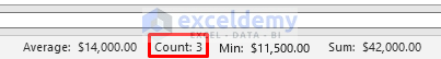
- The count of the colored cells appears at the bottom-right-hand side of the workbook.
Download Practice Workbook
To practice by yourself, download the following workbook.
<< Go Back to Colored Cells | Count Cells | Formula List | Learn Excel
Get FREE Advanced Excel Exercises with Solutions!

So no formulae to keep a running count of items that have broken the conditional formatting threshold preset?
It’s easy to check the count on hand, but I need to write a formulae so another table updates with the status of the conditional formatting thresholds.
Thank you VIRGIAL for your query. Yes, you can use the COUNTIF function to count the number of items that have broken the Conditional Formatting threshold value. For doing this, write down the following formula in your desired cell. (eg. D11)
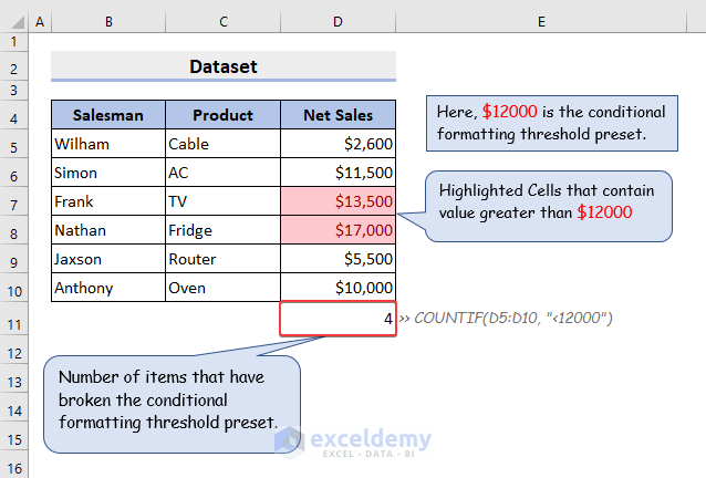
=COUNTIF(D5:D10, "<12000")Here, D5:D10 is the data range for which you want to set your condition and 12000 is the Conditional Formatting threshold value.
Additionally, the following image can be useful to comprehend the task.
hello,
Is there any method wherein one can count the number of conditional formatted color cells in row, one row at a time. formula based. each cells belongs to different column with conditional format for highlighting the Top/Bottom figures in respective columns as result the specific cell in the column gets highlighted depending on figure in that cell meeting the condition.
Been searching for answers/Tips in the net since a long time.
Regards
Thank you SHASHI, for your query. I think this article might help to solve your problem.
https://www.exceldemy.com/count-colored-cells-in-excel/#3_Utilizing_GETCELL_4_Macro_and_COUNTIFS_Functions
You can try to use this method for Conditional Formatted cells also. Further, if you have any confusion or query related to it, please let us know.