How to Count Colored Cells in Excel (4 Simple Ways)

Counting colored cells in Excel is needed for data analysis and visualization. By counting colored cells, we can quickly identify patterns and gain insights into the dataset. This feature is handy for tracking project statuses, validating data based on color-coded criteria, creating visual summaries for reporting, aiding decision-making and facilitating a deeper understanding of the data. But there isn’t any built-in function to count the colored cells in Excel.

In this Excel tutorial, you will learn how to count colored cells in Excel.

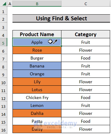
In this dataset, there are three categories: Fruit, Flower, and Food, each marked with a different color. Fruit is in Blue, Flower is in Orange, and Food has no background color. Now, let’s count the cells with a specific color, as shown in the GIF.

Here are 4 ways to count colored cells in Excel:

Using Find & Select Command

You can use the Find & Select command to count colored cells in each category. This provides a fast and effective method for analyzing data with specific visual characteristics.

To count colored cells in Excel using the Find & Select command:

1. Select the data range with colored cells.
2. Go to the Home tab > Editing group > Find & Select drop-down> Find.
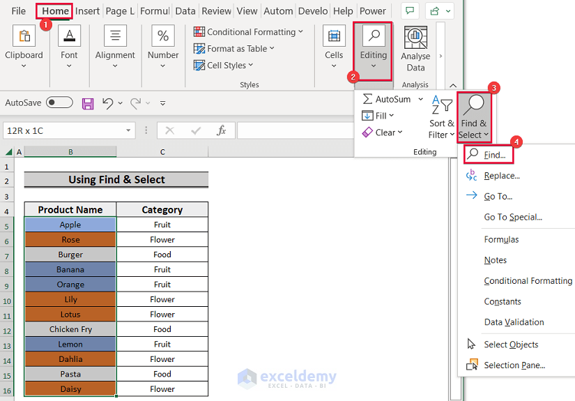
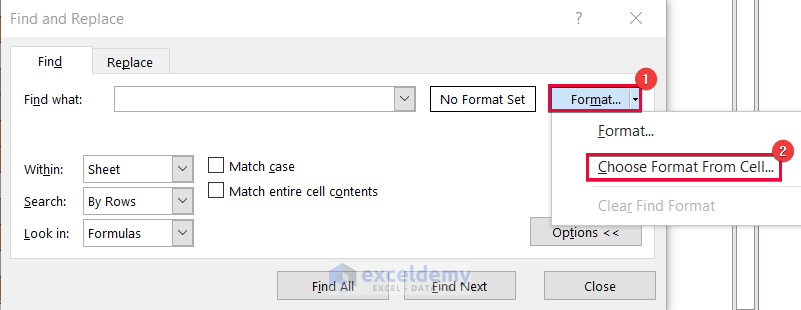
3. A Find and Replace dialogue box will pop up.
4. In the Find and Replace dialogue box:
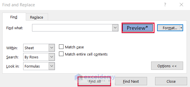
   • Click Options.
   • Format drop-down > Choose Format From Cell.

   A four-dimensional plus symbol will appear.

5. Place the plus symbol over any colored cell and click on it.
   We picked the color Blue.
   Again, the pop-up Find and Replace dialogue box will appear, and you will notice that the Preview* label box will be filled with a color similar to the color of the cell that you picked earlier.
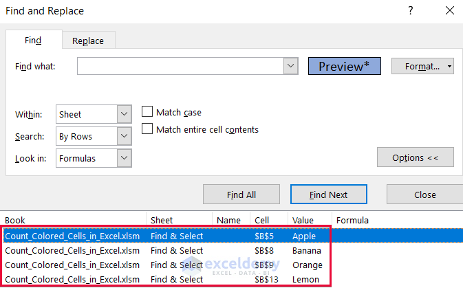
6. Select Find All.
   
7. Finally, you will get all the details of the specified colored cells, along with the count of those colored cells.

In the same way, you can count all the other colored cells in your worksheet in Excel.

Using SUBTOTAL Function and Filter Tool

The SUBTOTAL function counts the visible cells, and the Filter tool focuses on colored cells. It adjusts the count automatically when you modify the data or use various filters.

To count colored cells in Excel using the SUBTOTAL function and Filter tool:

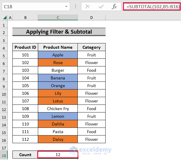
1. Select a blank cell below the data range.
2. Apply the formula: =SUBTOTAL(102,B5:B16)
   Here, the first argument set to 102 counts only the visible cells (hidden rows are excluded) in the given range. You will get the total count of the cells in the range.
   
3. Select only the headers of the data range.
4. Go to the Data tab > Filter.
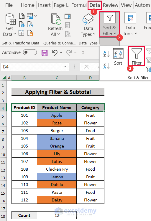
   It will insert a drop-down button in each header of the dataset.
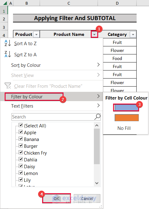
5. Click the drop-down button in the header of the column with colored cells.
6. Choose “Filter by Color” from the drop-down list to see all colors from your data range in a sub-list.
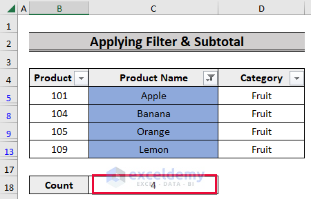
7. Click on the color you want to count.
   

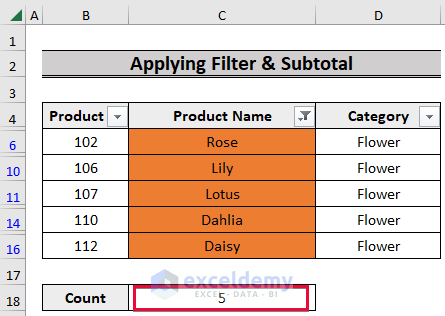
It will display only cells with the chosen color and show the count in the SUBTOTAL result cell.

In the same way, you can count all the other colored cells in your worksheet in Excel (e.g. when selecting the color Orange from the drop-down list, it shows the Orange-colored cells, and if there are 5 Orange cells in your dataset, the SUBTOTAL result cell will display 5).

Applying GET.CELL Macro4 and COUNTIFS Function

To count colored cells, combine the GET.CELL Macro 4 with the COUNTIFS function. GET.CELL Macro 4 gets cell color, and COUNTIFS counts cells based on different criteria, like color. The GET.CELL Macro 4 function only works on a named range in Excel.

Using Excel 4.0 Macro functions is limited because of compatibility issues and complexity. Also, it’s an older function and doesn’t have all the features of newer ones.

To count colored cells using GET.CELL Macro 4 function and COUNTIFS function:

Step 1: Create a Name Range

1. Go to Formulas tab > Define Names group > Define Name.
   
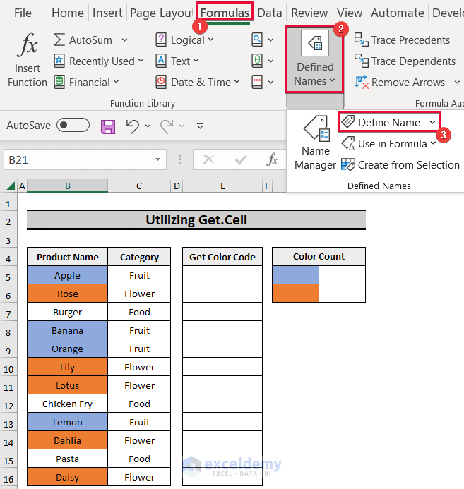
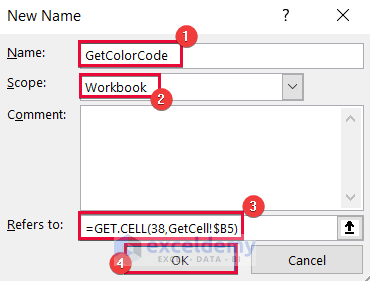
2. Next, in the New Name pop-up box, write the following:
   • Name: GetColorCode (this is a user-defined name)
   • Scope: Workbook
   • Refers to: =GET.CELL(38,GetCell!$B5)
     Here, 38 means the color of the referenced cell. GetCell means the sheet name that has your dataset. $B5 is the reference of the column with the background color.
   • Click OK.

   

Step 2: Find the Color Code for Each Cell

1. In the adjacent to the data, write the user-defined formula:=GetColorCode
2. Press Enter.
   
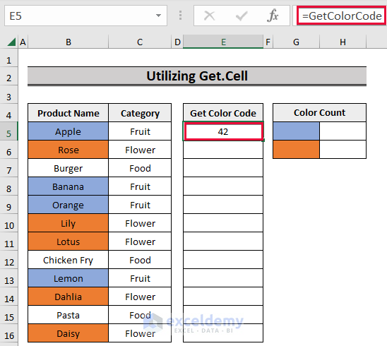
3. The formula will return a specific number specified in color.
4. Now, drag the cell down with the Fill Handle.
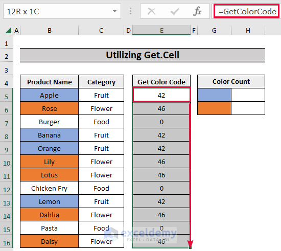
   All the cells with the same background color will get the same number, and if there is no background color, the formula will return 0.

Step 3: Apply COUNTIFS Function

1. Select the cell where you want to see the count of colored cells.
2. Apply the formula:=COUNTIFS($E5:$E$16,GetColorCode)
   Here, $E5:$E$16 is the range of the color code that we extracted from the user-defined formula.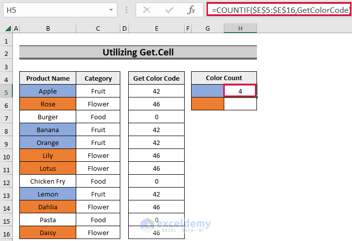As a result, you will get the count of the color-defined cells.
3. Again, click on the next cell.
4. Enter the following formula: =COUNTIFS($E5:$E$16,GetColorCode)As we have 5 cells colored Orange in our dataset, the user-defined GetColorCode formula gave us a count of 5.

Read More: Count Blank Colored Cells in Excel

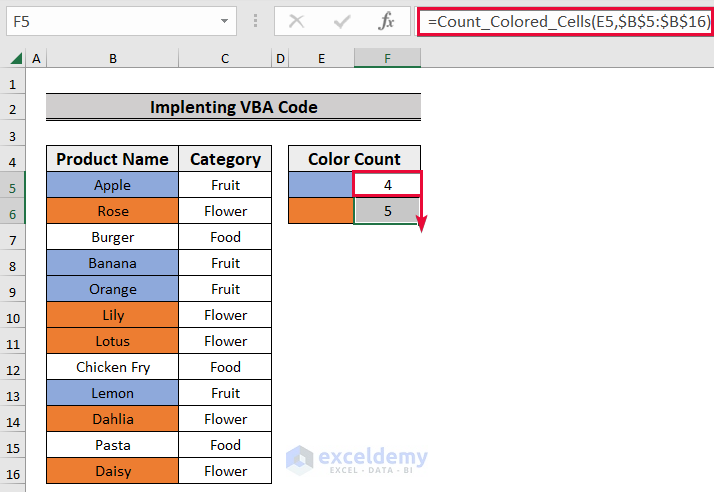
Using Excel VBA Code

VBA is the advancement of the Excel 4.0 macro. You can create a User-Defined Function using VBA. A user-defined function offers to use it as a regular function and is more flexible to use for new data.

To count colored cells in Excel using VBA:

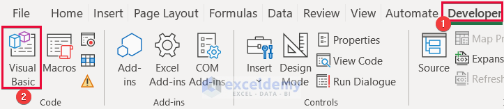
1. Go to Developer tab > Code group > Visual Basic to open the Visual Basic Editor. Or, press on ALT+F11.
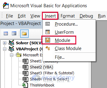
2. Navigate to the Insert tab > Module to create a new module for writing your code.
   
3. Copy and paste the following code:

   Function Count_Colored_Cells(ColorCells As Range, DataRange As Range)
   Dim Data_Range As Range
   Dim Cell_Color As Long
   Cell_Color = ColorCells.Interior.ColorIndex
   For Each Data_Range In DataRange
   If Data_Range.Interior.ColorIndex = Cell_Color Then
   Count_Colored_Cells = Count_Colored_Cells + 1
   End If
   Next Data_Range
   End Function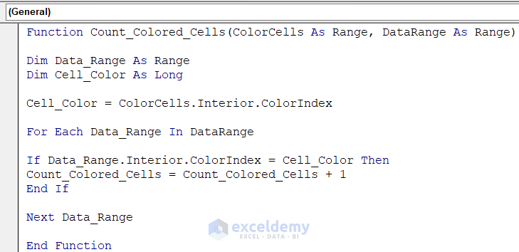

   This is not a Sub Procedure for the VBA program to run; this is creating a User Defined Function (UDF). So, after writing the code, don’t click the Run button from the menu bar.

4. Go back to the dataset and define cells with colors as we did in the previous method.
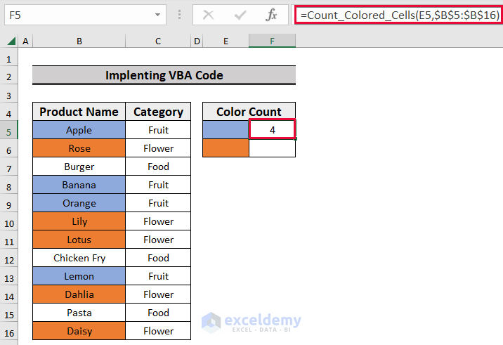
5. Write the following formula:=Count_Colored_Cells(E5,$B$5:$B$16)
   Here, Count_Colored_Cells is the user-defined function that you created in the VBA code. E5 is the color-defined cell and $B5:$B$16 is the range of the dataset with colored cells.
6. Press Enter.
   You can see the count of colored cells.
7. Drag down the cell using the Fill Handle tool.
   As we have 5 cells colored with Orange in our dataset, the user-defined Count_Colored_Cells function gave us the count 5.

Download Practice Template

You can download the free practice Excel template from here and practice on your own.

Conclusion

In conclusion, this article showed you 4 ways to count colored cells in Excel: use Find & Select, try SUBTOTAL with the Filter tool for dynamic counting, or apply Excel VBA coding for more advanced customization. These ways give you flexibility, offering efficient solutions to count colored cells in Excel based on individual needs, skills, and preferences. Feel free to comment if you have any questions regarding the topic.

Frequently Asked Questions

Is Excel VBA coding necessary to count colored cells?

No, VBA coding is not necessary, but it offers advanced customization options. Users with basic Excel skills can effectively count colored cells using simpler methods like formulas and filters.

Can I count colored cells in a specific range?

Yes, you can count colored cells in a specific range by adjusting the range parameter in your counting formula or method. This allows you to focus on a particular subset of your data.

Are there any limitations to counting colored cells in Excel?

While Excel provides various methods to count colored cells, these methods may have some limitations, such as compatibility issues or the need for adjustments when dealing with large datasets. It’s essential to choose a method that suits your specific requirements and constraints.

Count Colored Cells in Excel: Knowledge Hub

<< Go Back to Count Cells | Formula List | Learn Excel