Exclude Multiple Criteria in Same Column with SUMIFS Function

The SUMIFS function in Microsoft Excel evaluates the sum of a range of cells under multiple conditions. If you are looking for special tricks to exclude multiple criteria in the same column using the SUMIFS function in Excel, you’ve come to the right place. There are numerous ways to exclude multiple criteria in the same column using the SUMIFS function in Excel. This article will discuss the details of these methods. Let’s follow the complete guide to learn all of this.

Download Practice Workbook

Download this practice workbook to exercise while you are reading this article. It contains all the datasets in different spreadsheets for a clear understanding. Try it yourself while you go through the step-by-step process.

6 Suitable Examples to Exclude Multiple Criteria in Same Column Using SUMIFS Function

The following section will use six effective and tricky methods to exclude multiple criteria in the same column using the SUMIFS function in Excel. This section provides extensive details on these methods. You should learn and apply these to improve your thinking capability and Excel knowledge. We use the Microsoft Office 365 version here, but you can utilize any other version according to your preference.

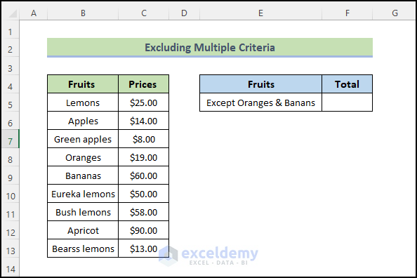
1. Excluding Multiple Criteria

Here, we will demonstrate how to exclude multiple criteria in the same column using the SUMIFS function. For this example, let’s assume we have a dataset of some fruits with their prices. Now we will show how to find the total costs of all the fruits except Oranges and Bananas.

Let’s walk through the following steps to do the task.

📌 Steps:

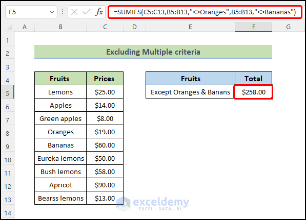
• First of all, select the cell you want to put the value in (cell F5).
• Then write down the following formula in it.

The SUMIFS function finds the rows of fruits except for oranges and bananas. As soon as the matched rows are found, the prices are added up and a result is displayed.

• Next, press Enter.
• Consequently, you will get the total prices in cell F5.

Read More: How to Use SUMIFS Function in Excel with Multiple Criteria

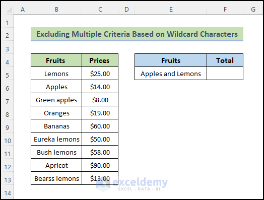
2. Excluding Multiple Criteria Based on Wildcard Characters

Use of the wildcard characters (*,?, ) will enable you to locate the precise text value that you might not be able to recall right away. For instance, we are interested in the total costs of some fruits whose names begin with “Apples” and “Lemons”. For the purpose of calculation, we will combine SUM and SUMIFS functions.

Let’s walk through the following steps to do the task.

📌 Steps:

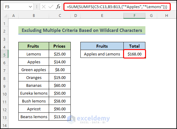
• First of all, select the cell you want to put the value in (cell F5).
• Then write down the following formula in it.

• Next, press Enter.
• Consequently, you will get the total prices in cell F5.

Read More: SUMIFS with Wildcard in Excel (+ Alternative Formulas)

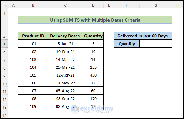
3. Using SUMIFS with Multiple Dates Criteria

We will now show you how to use dates by applying TODAY and SUMIFS functions. Consider for the purposes of this example that we have a dataset of some fruits with the delivery date and quantity. We’ll now give an example of how to calculate the total number of deliveries made over the previous 60 days.

Let’s walk through the following steps to do the task.

📌 Steps:

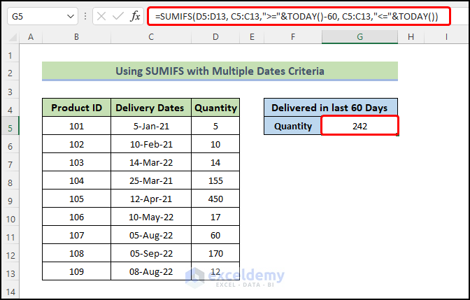
• First of all, select the cell you want to put the value in (cell G5).
• Then write down the following formula in it.

• Next, press Enter.
• Consequently, you will get the total quantity in cell G5.

Read More: How to Use SUMIFS with Date Range and Multiple Criteria (7 Quick Ways)

Similar Readings

• Excel SUMIFS with Multiple Vertical and Horizontal Criteria
• How to Use SUMIFS Formula with Multiple Criteria in Excel (11 Ways)
• SUMIFS with INDEX-MATCH Formula Including Multiple Criteria
• How to Apply SUMIFS with INDEX MATCH for Multiple Columns and Rows

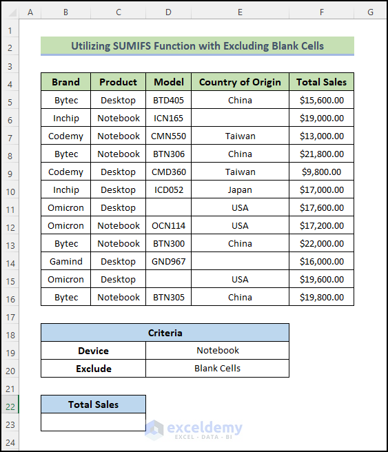
4. Utilizing SUMIFS Function with Excluding Blank Cells

There may occasionally be some empty cells in our dataset or table. Use the ‘Not Equal to’ operator (>) as the criteria for a range if you want to eliminate rows with empty cells. Now, using our dataset, we can determine the total sales value of the laptops that are present in the table with sufficient and complete data.

Let’s walk through the following steps to do the task.

📌 Steps:

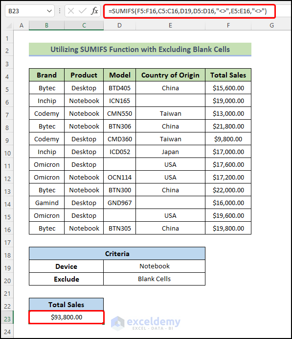
• First of all, select the cell you want to put the value in (cell B25).
• Then write down the following formula in it.

• Next, press Enter.
• Consequently, you will get the total sales in cell B25.

Read More: Excel SUMIFS Not Equal to Multiple Criteria (4 Examples)

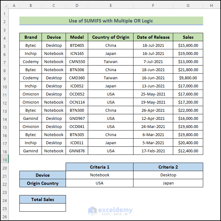
5. Use of SUMIFS with Multiple OR Logic

In some cases, we may need to extract the sum for multiple criteria that cannot be handled using only the SUMIFS function. For multiple criteria, we can simply add two or more SUMIFS functions. As an example, we would like to calculate the sum of all notebooks and desktops originating in the USA and Japan.

Let’s walk through the following steps to do the task.

📌 Steps:

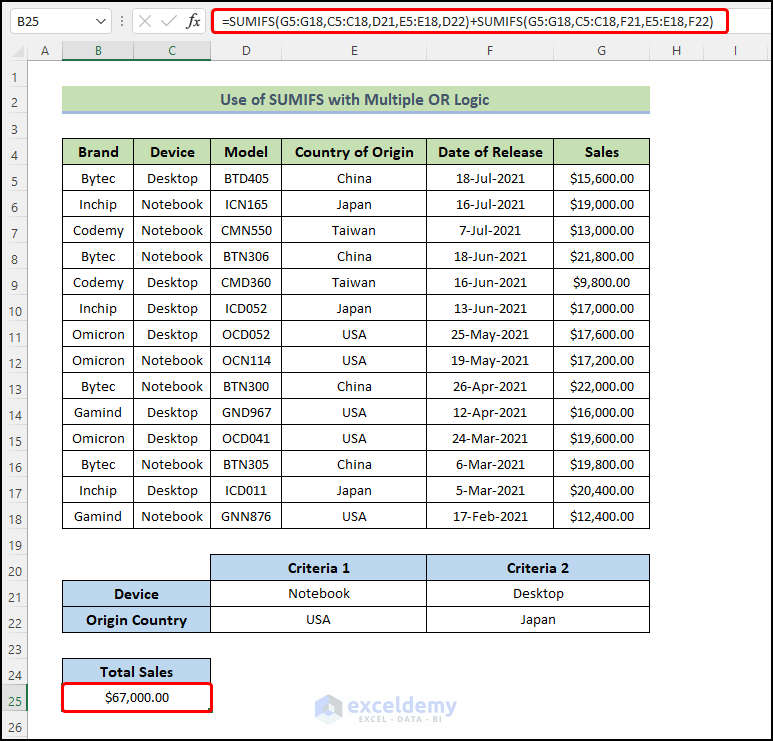
• First of all, select the cell you want to put the value in (cell B25).
• Then write down the following formula in it.

• Next, press Enter.
• Consequently, you will get the total sales in cell B25.

Read More: Excel SUMIFS with Multiple Sum Ranges and Multiple Criteria

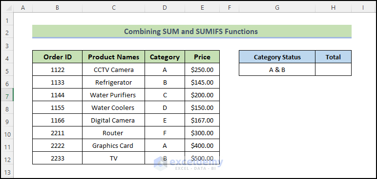
6. Combining SUM and SUMIFS Functions

The dataset we have here contains details of an order for a company. There are four attributes in the table: Order ID, Product Names, Category, and Price.  As an example, let’s count the total prices where the category status is A and B. For the purpose of calculation, we will combine SUM and SUMIFS functions.

Let’s walk through the following steps to do the task.

📌 Steps:

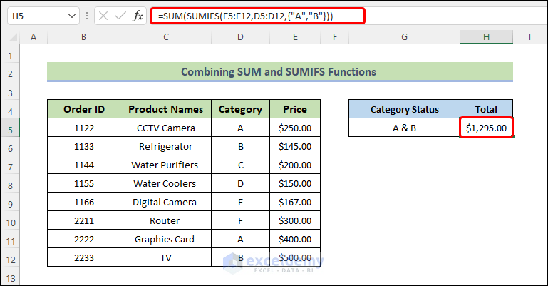
• First of all, select the cell you want to put the value in (cell H5).
• Then write down the following formula in it.

• Next, press Enter.
• Consequently, you will get the total sales in cell H5.

Read More: How to Use VBA Sumifs with Multiple Criteria in Same Column

💬 Things to Remember

✎ If you input an array condition into SUMIFS and at the same time it finds a merged cell as the return destination, it will return #SPILL error.

✎ The function will return zero(0) instead of showing an error unless you use the Double-Quotes(““) outside a text value as range criteria. Therefore, you should be careful when entering text values as criteria inside the SUMIFS function.

Conclusion

That’s the end of today’s session. I strongly believe that from now, you may be able to exclude multiple criteria in the same column using the SUMIFS function in Excel. If you have any queries or recommendations, please share them in the comments section below.

Don’t forget to check our website ExcelDemy.com for various Excel-related problems and solutions. Keep learning new methods and keep growing!

Related Articles

• SUMIFS Sum Range Multiple Columns in Excel(6 Easy Methods)
• [Fixed]: SUMIFS Not Working with Multiple Criteria (3 Solutions)
• SUMIFS with Multiple Criteria Along Column and Row in Excel
• How to Use SUMIFS When Cells Are Not Equal to Multiple Text
• SUMIFS with Multiple Criteria in the Same Column (5 Ways)