Method 1 – Apply the SUMIFS Function with Comparison Operators
We are going to sum all the values greater than a given benchmark from a subset of the table (the criteria value). Our criteria value is in cell H4, and the comparison value is in cell H5.

Steps:
- Select cell H6.
- Use the following formula in the cell.
=SUMIFS(D5:D15,C5:C15,H4,D5:D15,H5)
- Press Enter.
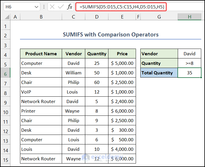
- You will get the sum result.
Read More: How to Use SUMIFS with Multiple Criteria in the Same Column
Method 2 – Using the SUMIFS Function with a Date Value
We have added a new column F for Delivery Date. Our vendor criteria value will be in cell I4. We will sum how many items have already been delivered or will be delivered in the next 20 days.
Steps:
- Select cell I5.
- Use the following formula in the cell.
=SUMIFS(D5:D15, F5:F15,">="&TODAY()-20, F5:F15,"<="&TODAY(),C5:C15,I4)
- Press Enter.
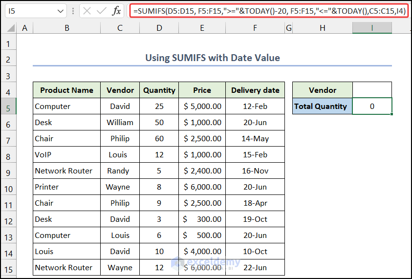
- It will show you zero (0) in cell I5.
- Insert the vendor criteria in cell I4. We wrote David.
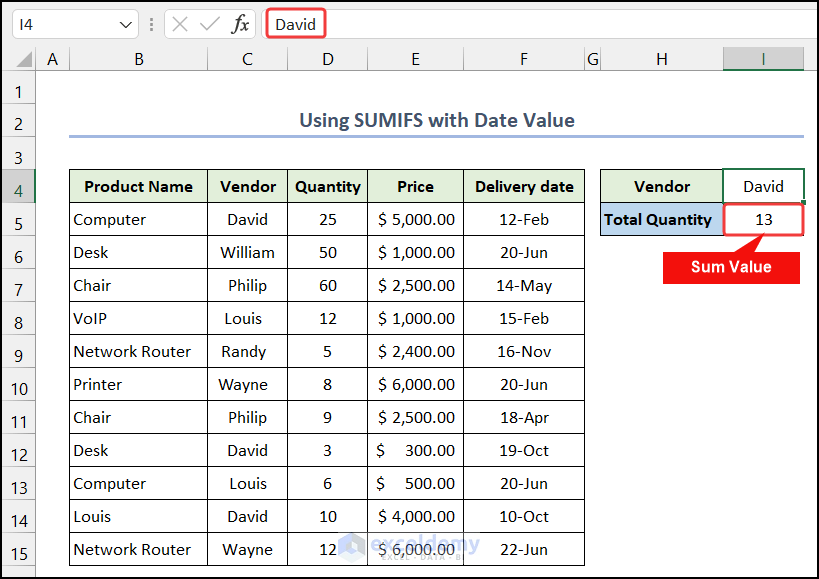
- The formula sums up the quality of the product which lies within our time limit.
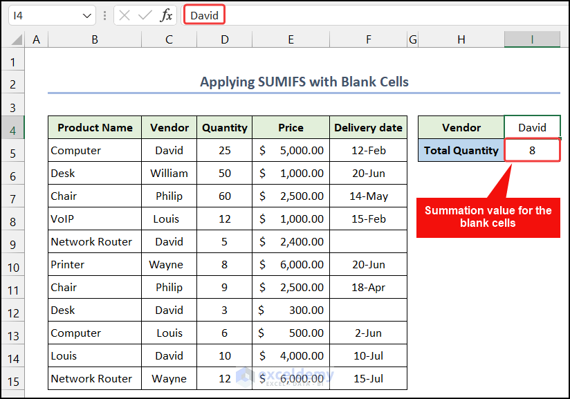
Method 3 – Applying the SUMIFS Function for Blank Cells
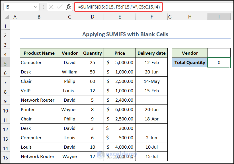
We have 4 entities for vendor David. Among them, 2 delivery dates are blank cells. We’ll sum the number of items for those sales.
Steps:
- Select cell I5.
- Insert the following formula inside the cell.
=SUMIFS(D5:D15, F5:F15,"=",C5:C15,I4)
- Press Enter, and you will get a 0 value in that cell.
- Write down David as the vendor criteria in cell I4.
- The formula will sum up the quality of the product for the blank cells, and the other two cells will be omitted.
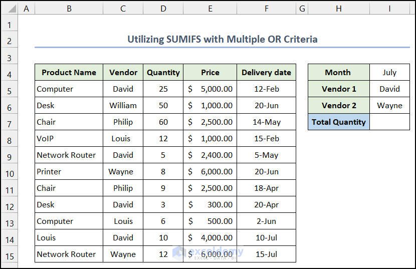
Method 4 – Utilizing the SUMIFS Function with Multiple OR Criteria
We’ll sum up the sales for multiple vendors in a given month.
Steps:
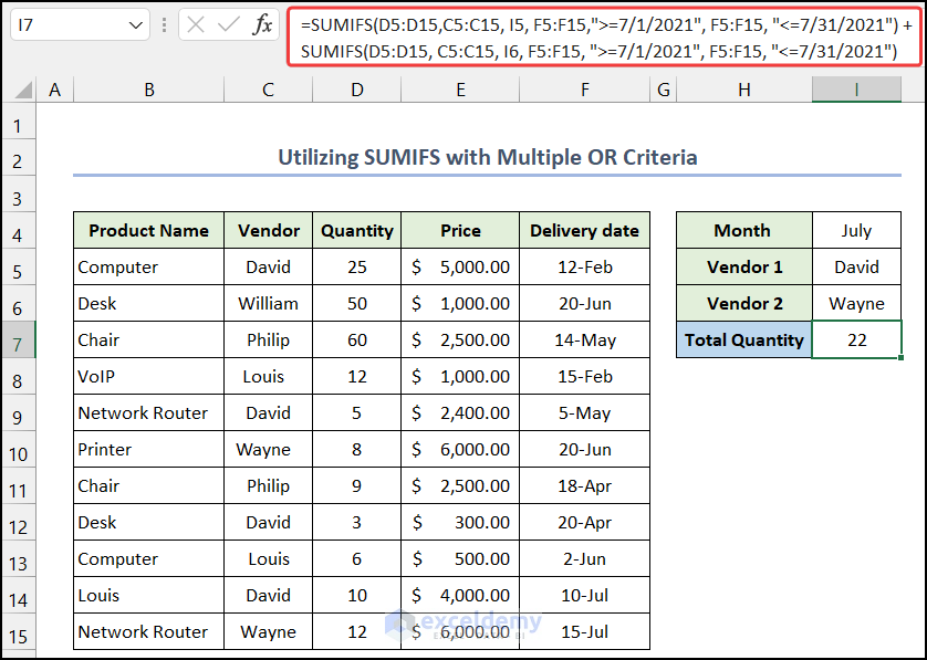
- Select cell I7.
- Insert the following formula inside the cell.
=SUMIFS(D5:D15,C5:C15, I5, F5:F15,">=7/1/2021", F5:F15, "<=7/31/2021") + SUMIFS(D5:D15, C5:C15, I6, F5:F15, ">=7/1/2021", F5:F15, "<=7/31/2021")
- Press Enter.
Breakdown of the Formula
SUMIFS(D5:D15,C5:C15, I5, F5:F15,”>=7/1/2021″, F5:F15, “<=7/31/2021”): The SUMIF function sums up all the values between our criteria. Here, the value is 10.
SUMIFS(D5:D15, C5:C15, I6, F5:F15, “>=7/1/2021”, F5:F15, “<=7/31/2021”): The SUMIF function sums up all the values defined in our another criterion. Here, the value is 12.
SUMIFS(D5:D15,C5:C15, I5, F5:F15,”>=7/1/2021″, F5:F15, “<=7/31/2021”) + SUMIFS(D5:D15, C5:C15, I6, F5:F15, “>=7/1/2021”, F5:F15, “<=7/31/2021”): Finally, the addition operator add both values and show it in cell I7. Here, the value is 22.
Read More: Excel SUMIFS with Multiple Vertical and Horizontal Criteria
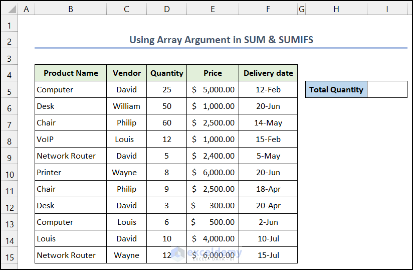
Method 5 – Using an Array Argument in SUM and SUMIFS Functions
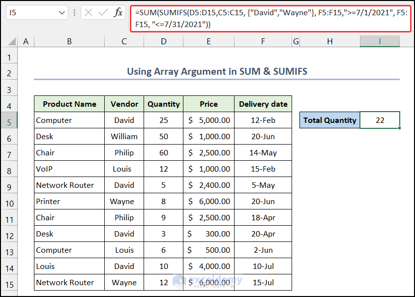
Let’s add up the sales for two vendors, David and Wayne for July.
Steps:
- Select I5.
- Insert the following formula inside the cell.
=SUM(SUMIFS(D5:D15,C5:C15, {"David","Wayne"}, F5:F15,">=7/1/2021", F5:F15, "<=7/31/2021"))
- Press Enter.
Breakdown of the Formula
SUMIFS(D5:D15,C5:C15, {“David”,”Wayne”}, F5:F15,”>=7/1/2021″, F5:F15, “<=7/31/2021”): The SUMIF function figure out the values validated between our criteria. Here, the value is 10, 12.
SUM(SUMIFS(D5:D15,C5:C15, {“David”,”Wayne”}, F5:F15,”>=7/1/2021″, F5:F15, “<=7/31/2021”)): At last, the SUM function adds both values get by the SUMIF function. Here, the value is 22.
Read More: SUMIFS: Sum Range Across Multiple Columns
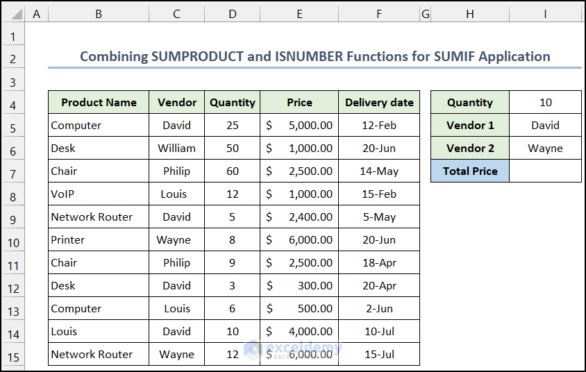
Method 6 – Combining SUMPRODUCT, ISNUMBER, and MATCH Functions for SUMIF
Our criteria are in the range of cells I4:I6. Here, we will determine the Total Price for our criteria.
Steps:
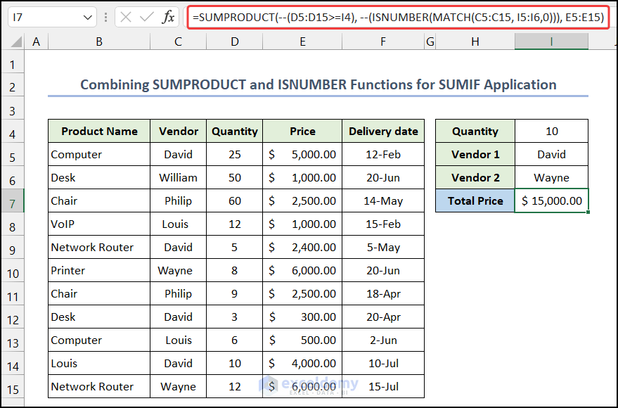
- Select cell I7.
- Use the following formula inside the cell.
=SUMPRODUCT(--(D5:D15>=I4), --(ISNUMBER(MATCH(C5:C15, I5:I6,0))), E5:E15)
- Press Enter.
Breakdown of the Formula
MATCH(C5:C15, I5:I6,0): The MATCH function will check the criteria and define them with 1 and 2. Here, we get three 1 for David and one 2 for Wayne.
ISNUMBER(MATCH(C5:C15, I5:I6,0)): The ISNUMBER function checks the result of the MATCH function. If the result is numeric, it will show TURE. Otherwise, it will display FALSE.
SUMPRODUCT(–(D5:D15>=I4), –(ISNUMBER(MATCH(C5:C15, I5:I6,0))), E5:E15): Finally, the SUMPRODUCT function sum the total price. Here, the value is $15,000.00.
Read More: How to Apply SUMIFS with INDEX MATCH for Multiple Columns and Rows
Things to Remember
- In Excel, the order of arguments of the SUMIF and SUMIFS functions are different. In particular, sum_range is the first parameter in SUMIFS, but it is the third in SUMIF.
- In the SUMIFS function, you need an equal number of ranges and criteria applied to them.
Download the Practice Workbook
Related Articles
- SUMIFS with Multiple Criteria Along Column and Row in Excel
- Exclude Multiple Criteria in Same Column with SUMIFS Function
- How to Use VBA SUMIFS with Multiple Criteria in Same Column
<< Go Back to Excel SUMIFS with Multiple Criteria | Excel SUMIFS Function | Excel Functions | Learn Excel
Get FREE Advanced Excel Exercises with Solutions!
