Suppose you have the following dataset.
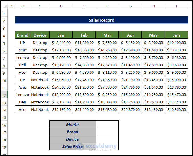
Method 1 – SUMIFS with INDEX-MATCH Combining Multiple Criteria
Steps
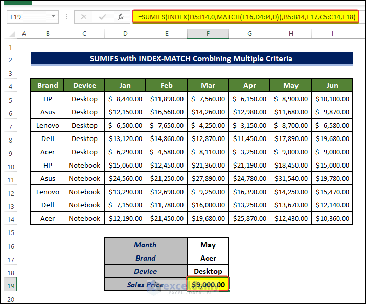
- Select an appropriate cell (F19 in this example) and enter the following formula:
=SUMIFS(INDEX(D5:I14,0,MATCH(F16,D4:I4,0)),B5:B14,F17,C5:C14,F18)
Formula Breakdown
MATCH(F16,D4:I4,0)
In this example, the formula will search for the values mentioned in cell F16 in the range of cell D4:I4, and return the column rank in that list.
INDEX(D5:I14,0,MATCH(F16,D4:I4,0))
The function will return the cell address of all the rows in the column returned in the MATCH formula, in the mentioned range cells D5:I14. The output, in this case, is H5:H14.
SUMIFS(INDEX(D5:I14,0,MATCH(F16,D4:I4,0)),B5:B14,F17,C5:C14,F18)
The formula will sum the range value returned by the INDEX formula, only if the F17 value is present in the range of cells B5:B14. If the value is not present in any row, the corresponding row value in the range of cell H5:H14 will be ignored. After it satisfies the first criterion, it will move to the second criterion—the value of F18 in the range of cell C5:C18, only if the F18 value is present corresponding in the range of cells C5:C14.
Read More: Excel SUMIFS with Multiple Sum Ranges and Multiple Criteria
Method 2 – Using SUMIFS with INDEX-MATCH Excluding Blank Cells
Steps
In the dataset, H9 is now blank.
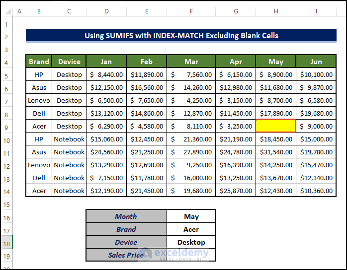
- Select an appropriate cell (F19) and enter the following formula:
=SUMIFS(INDEX(D5:I14,0,MATCH(F16,D4:I4,0)),B5:B14,"<>",C5:C14,"<>")

Formula Breakdown
MATCH(F16,D4:I4,0)
In this example, the formula will search for the values mentioned in cell F16 in the range of cell D4:I4, and return the column rank in that list.
INDEX(D5:I14,0,MATCH(F16,D4:I4,0))
The formula will return the cell address of all the rows in the column returned in the MATCH formula, in the mentioned range cells D5:I14. The output, in this case, is H5:H14.
SUMIFS(INDEX(D5:I14,0,MATCH(F16,D4:I4,0)),B5:B14,”<>”,C5:C14,”<>”)
The formula will sum the range value returned by the INDEX formula. The summation will occur if there is no blank cell in the range of cells B5:B14 and C5:C14. The “<>” would set the argument in this way.
Method 3 – Combining Multiple SUMIFS with INDEX-MATCH Using OR Logic
Steps
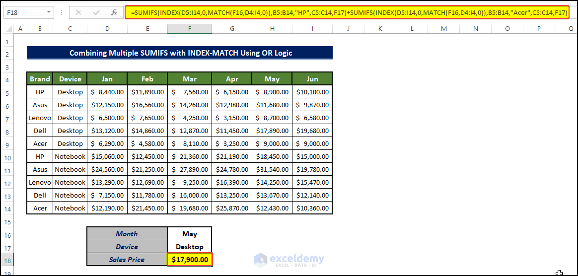
- Select a relevant cell (F18) and enter the following formula:
=SUMIFS(INDEX(D5:I14,0,MATCH(F16,D4:I4,0)),B5:B14,"HP",C5:C14,F17)+SUMIFS(INDEX(D5:I14,0,MATCH(F16,D4:I4,0)),B5:B14,"Acer",C5:C14,F17)
Formula Breakdown
MATCH(F16,D4:I4,0)
The formula will search for the values mentioned in cell F16 in the range of cell D4:I4, and return the column rank in that list.
INDEX(D5:I14,0,MATCH(F16,D4:I4,0))
The formula will return the cell address of all of the rows in the column returned in the MATCH formula, in the mentioned range cells D5:I14. The output, in this case, is H5:H14.
SUMIFS(INDEX(D5:I14,0,MATCH(F16,D4:I4,0)),B5:B14,”HP”,C5:C14,F17)+SUMIFS(INDEX(D5:I14,0,MATCH(F16,D4:I4,0)),B5:B14,”Acer”,C5:C14,F17)
The first part before the + sign indicates the summation of values from the range returned from the INDEX formula if “HP” is present in the range of cell C5:C14. After the plus sign, the structure remains the same, just the HP is replaced with Acer. Both section values are then added together.
Read More:
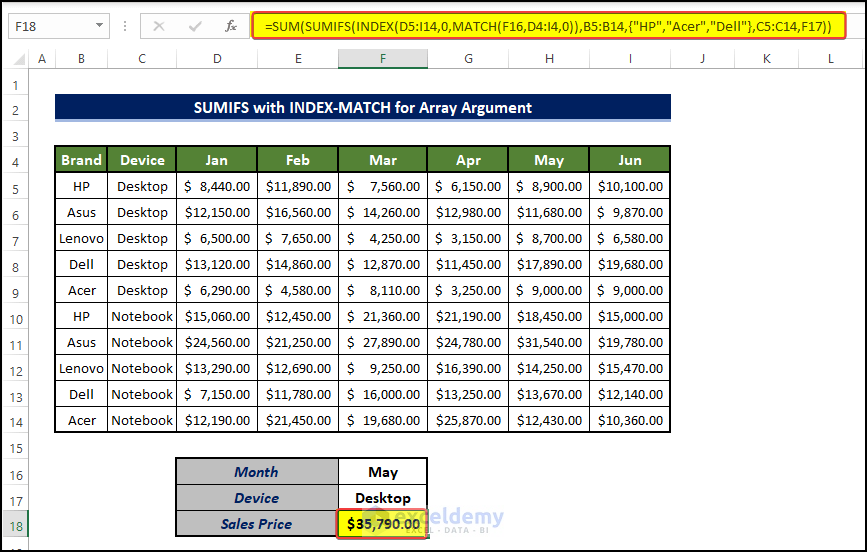
Method 4 – SUMIFS with INDEX-MATCH for Array Argument
Steps
- Select a relevant cell (F18), and enter the following formula:
=SUM(SUMIFS(INDEX(D5:I14,0,MATCH(F16,D4:I4,0)),B5:B14,{"HP","Acer","Dell"},C5:C14,F17))
Formula Breakdown
MATCH(F16,D4:I4,0)
This formula will search for the values mentioned in cell F16 in the range of cell D4:I4, and return the column rank in that list.
INDEX(D5:I14,0,MATCH(F16,D4:I4,0))
This formula will return the cell address of all of the rows in the column returned in the MATCH formula, in the mentioned range cells D5:I14. The output, in this case, is H5:H14.
SUM(SUMIFS(INDEX(D5:I14,0,MATCH(F16,D4:I4,0)),B5:B14,{“HP”,”Acer”,”Dell”},C5:C14,F17))
The formula will sum values in the range only if the “HP”, “Acer”, and “Dell” values are present in the range of cells B5:B14. If the value is not present in any row, the corresponding row value in the range of cell H5:H14 will be ignored. After it satisfies the first criterion, it will move to the second criterion, and so on. It will be for the value of F18 in the range of cell C5:C18. They would sum value in the range of H5:H14 only if the F18 value is present corresponding in the range of cells C5:C14.
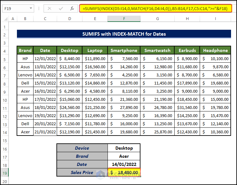
Method 5 – SUMIFS with INDEX-MATCH for Dates
Steps
- Then select the correct cell (F19) and enter the following formula:
=SUMIFS(INDEX(D5:I14,0,MATCH(F16,D4:I4,0)),B5:B14,F17,C5:C14,">="&F18)
Formula Breakdown
MATCH(F16,D4:I4,0)
The formula will search for the values mentioned in cell F16 in the range of cell D4:I4, and return the column rank in that list.
INDEX(D5:I14,0,MATCH(F16,D4:I4,0))
The formula will return the cell address of all the rows in the column returned in the MATCH formula, in the mentioned range cells D5:I14. The output, in this case, is H5:H14.
SUMIFS(INDEX(D5:I14,0,MATCH(F16,D4:I4,0)),B5:B14,F17,C5:C14,F18)
The formula will sum values in the range only if the F17 value is present in the range of cells B5:B14. If the value is not present in any row, the corresponding row value in the range of cell H5:H14 will be ignored. After it satisfies the first criterion, it will move to the second criterion. The criteria here are data-related. If the values are after the date mentioned in cell F18, then they are going to be summed.
Method 6 – SUMIFS with INDEX-MATCH Using Comparison Operator
Steps
- Then select the appropriate cell (F19) and enter the following formula:
=SUMIFS(INDEX(D5:I14,0,MATCH(F16,D4:I4,0)),B5:B14,F17,INDEX(D5:I14,0,MATCH(F16,D4:I4,0)),">=10000")

Formula Breakdown
MATCH(F16,D4:I4,0)
This formula will search for the values mentioned in cell F16 in the range of cell D4:I4. And return the column rank in that list.
INDEX(D5:I14,0,MATCH(F16,D4:I4,0))
This formula will return the cell address of all of the rows in the column returned in the MATCH formula, in the mentioned range cells D5:I14. The output, in this case, is H5:H14.
SUMIFS(INDEX(D5:I14,0,MATCH(F16,D4:I4,0)),B5:B14,F17,INDEX(D5:I14,0,MATCH(F16,D4:I4,0)),”>=10000″)
The formula will sum value in the range only if the F17 value is present in the range of cells B5:B14. If the value is not present in any row, the corresponding row value in the range of cell H5:H14 will not count. After it satisfies the first criterion, it will move to the second criterion. For the values, only those that are over 10,000 will be added. The last part of the formula ensures this.
Download Practice Workbook
Download this practice workbook below.
Related Articles
- How to Use SUMIFS Function with Multiple Sheets in Excel
- Excel SUMIFS Not Equal to Multiple Criteria
- How to Use SUMIFS Function with Wildcard in Excel
- SUMIFS Not Working with Multiple Criteria
<< Go Back to Excel SUMIFS with Multiple Criteria | Excel SUMIFS Function | Excel Functions | Learn Excel
Get FREE Advanced Excel Exercises with Solutions!
