Method 1 – Multiple Sum Ranges & Criteria with Excel SUMIFS Function Using Comparison Operators
Steps:
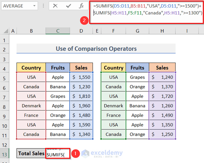
- Go to the cell where you want to insert the result (cell C13 in our case).
- To sum up the Sales values, type the formula:
=SUMIFS(D5:D11,B5:B11,"USA",D5:D11,">=1500")+SUMIFS(H5:H11,F5:F11,"Canada",H5:H11,">=1300")- We can see the formula in the Formula Bar of the image below.
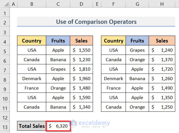
- After inserting the formula, press the Enter key to get the result.
- We can see the output in cell C13 of the screenshot below.
How Does the Formula Work?
- D5:D11 & H5:H11 (first part): Indicate the sum_range.
- B5:B11 & F5:F11: Denote the criteria_range1.
- “USA” & “Canada”: Refer to the criteria1.
- D5:D11 & H5:H11 (last part): Denote the criteria_range2.
- “>=1500” & “>=1300”: Refer to the criteria2.
- SUMIFS(D5:D11,B5:B11,”USA”,D5:D11,”>=1500″): Returns the summation of the Sales for USA with the Sales value greater than $1500.
- SUMIFS(H5:H11,F5:F11,”Canada”,H5:H11,”>=1300″): Adds the Sales values for Canada that are greater than $1300.
- SUMIFS(D5:D11,B5:B11,”USA”,D5:D11,”>=1500″)+SUMIFS(H5:H11,F5:F11,”Canada”,H5:H11,”>=1300″): Sums up the two values gained from the two SUMIFS formula.
Method 2 – Including Dates in the SUMIFS Function with Multiple Sum Ranges and Criteria
Steps:
- Activate cell C13 to place the summation.
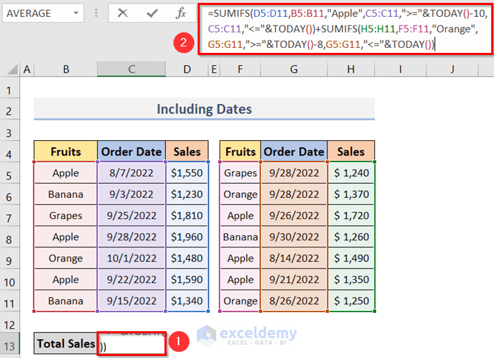
- Insert the following formula in the cell (C13) for adding the Sales values:
=SUMIFS(D5:D11,B5:B11,"Apple",C5:C11,">="&TODAY()-10,C5:C11,"<="&TODAY())+SUMIFS(H5:H11,F5:F11,"Orange",G5:G11,">="&TODAY()-8,G5:G11,"<="&TODAY())- See the formula in the Formula Bar of the picture below.
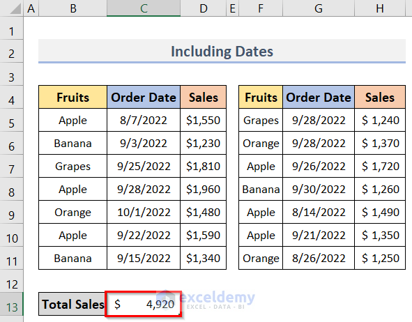
- Press the Enter key to find the result.
- See the output in cell C13 of the screenshot below.
How Does the Formula Work?
- &TODAY: Returns the current date.
- SUMIFS(D5:D11,B5:B11,”Apple”,C5:C11,”>=”&TODAY()-10,C5:C11,”<=”&TODAY()): Adds the Sales for Apple with the Order Dates within 10 days before & including the current date.
- SUMIFS(H5:H11,F5:F11,”Orange”,G5:G11,”>=”&TODAY()-8,G5:G11,”<=”&TODAY()): Sums up the Sales for Orange with the Order Dates within 8 days before & including the current date.
- SUMIFS(D5:D11,B5:B11,”Apple”,C5:C11,”>=”&TODAY()-10,C5:C11,”<=”&TODAY())+SUMIFS(H5:H11,F5:F11,”Orange”,G5:G11,”>=”&TODAY()-8,G5:G11,”<=”&TODAY()): Returns the summation of the two values gained from the two SUMIFS formula.
Method 3 – Array Argument for Multiple Sum Ranges and Criteria with SUM & SUMIFS Functions
Steps:
- Select cell C13.
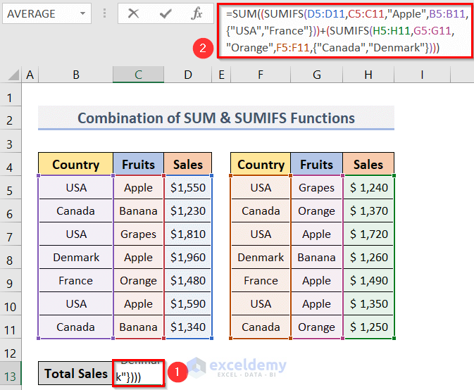
- To add the Sales values, insert the following formula in cell C13:
=SUM((SUMIFS(D5:D11,C5:C11,"Apple",B5:B11,{"USA","France"}))+(SUMIFS(H5:H11,G5:G11,"Orange",F5:F11,{"Canada","Denmark"})))- We can see the formula in the Formula Bar of the image below.
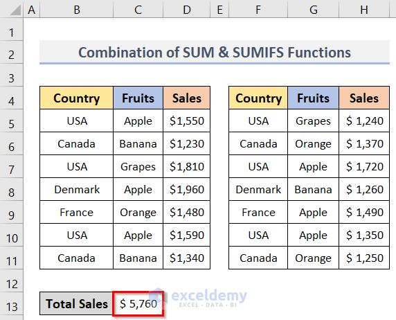
- Press Ctrl + Shift + Enter (for array formula).
How Does the Formula Work?
- SUMIFS(D5:D11,C5:C11,”Apple”,B5:B11,{“USA”,”France”}): Returns two summations of the Sales of Apple. The first one is for the orders by the USA and the second one is for France.
- SUMIFS(H5:H11,G5:G11,”Orange”,F5:F11,{“Canada”,”Denmark”}): Returns two summations of the Sales of Orange. The first one is for the USA and the second one is for France.
- SUM((SUMIFS(D5:D11,C5:C11,”Apple”,B5:B11,{“USA”,”France”}))+(SUMIFS(H5:H11,G5:G11,”Orange”,F5:F11,{“Canada”,”Denmark”}))): Returns the summation of the four values obtained from the two SUMIFS formula.
- We can see the result in cell C13 of the screenshot below.
Method 4 – Using SUMIFS Function for Blank & Non-Blank Cells with Multiple Ranges & Criteria
Steps:
- Select the cell (C13) where you want to insert the summation.
- To get the summation of the Sales, type the following formula:
=SUMIFS(E5:E11,B5:B11,"USA",C5:C11,"<>",D5:D11,"=")+SUMIFS(J5:J11,G5:G11,"Canada",H5:H11,"<>",I5:I11,"=")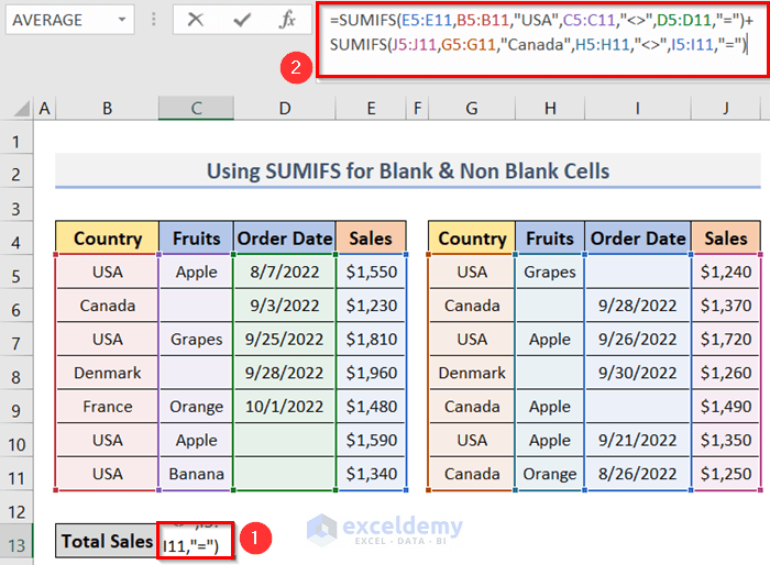
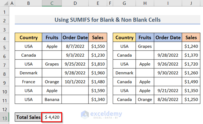
- Get the result by pressing the Enter key (see screenshot).
How Does the Formula Work?
- “<>”: Indicates the non-blank cells.
- “=”: Denotes the blank cells.
- SUMIFS(E5:E11,B5:B11,”USA”,C5:C11,”<>”,D5:D11,”=”): Adds the Sales for USA with the non-blank cells in the C5:C11 range and the blank cells in the D5:D11 range.
- SUMIFS(J5:J11,G5:G11,”Canada”,H5:H11,”<>”,I5:I11,”=”): Sums up the Sales for Canada with the non-blank cells in the H5:H11 range and the blank cells in the I5:I11 range.
- SUMIFS(E5:E11,B5:B11,”USA”,C5:C11,”<>”,D5:D11,”=”)+SUMIFS(J5:J11,G5:G11,”Canada”,H5:H11,”<>”,I5:I11,”=”): Returns the summation of the two values gained from the two SUMIFS formula.
Method 5 – Utilizing SUMIFS Function for Dynamic Criteria with Named Range
Steps:
- Select the range C13:C14 to create the dynamic criteria.
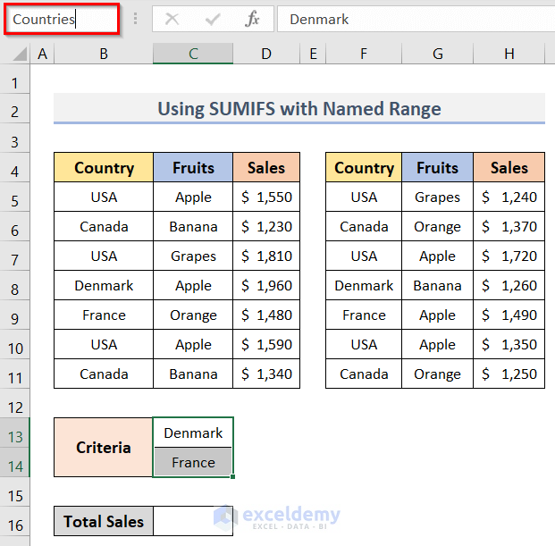
- Go to the Name Box (see screenshot).
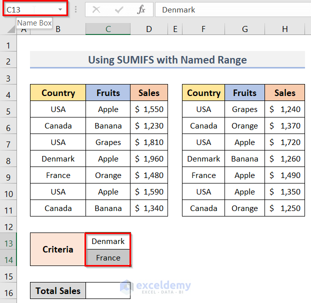
- Type any name (Countries) in the Name Box for the dynamic criteria.
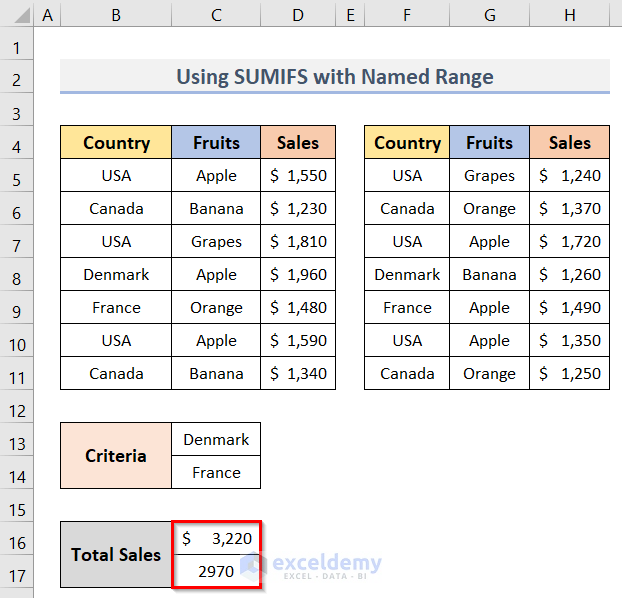
- Select cell C16 where you want to keep the output.
- When you start inserting the formula and typing dynamic criteria (Countries). You will see it as a suggestion (see screenshot).
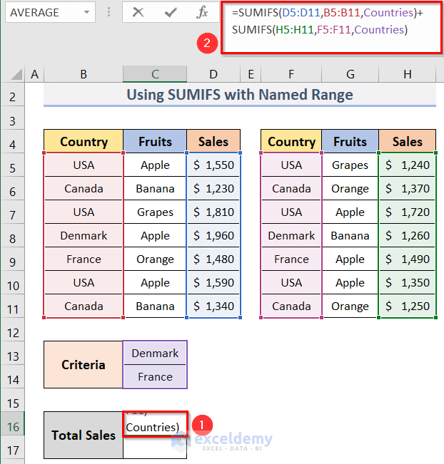
- The formula is:
=SUMIFS(D5:D11,B5:B11,Countries)+SUMIFS(H5:H11,F5:F11,Countries)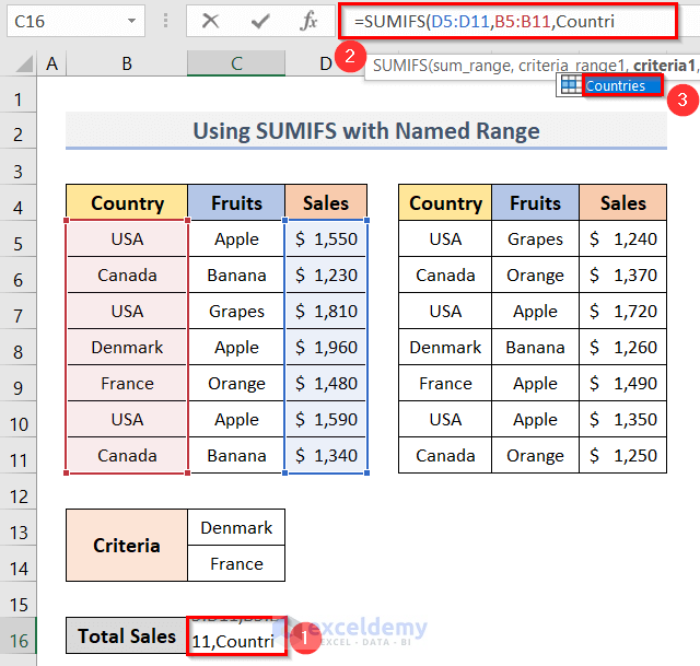
- Finish typing the formula to find the output.
- After pressing Ctrl + Shift + Enter (for the older versions before Excel 2019), you will get the output in cells C16 and C17.
- The value in cell C16 is the summation of Sales for Denmark, and the one in C17 is for France.
How Does the Formula Work?
- SUMIFS(D5:D11,B5:B11,Countries): Adds the Sales for the range B5:B11 based on the dynamic criteria (Countries).
- SUMIFS(H5:H11,F5:F11,Countries): Sums up the Sales for the range H5:H11 based on the dynamic criteria named Countries.
- SUMIFS(D5:D11,B5:B11,Countries)+SUMIFS(H5:H11,F5:F11,Countries): Returns the summation of the two values gained from the two SUMIFS formula.
Method 6 – Applying Wildcard Character with SUMIFS Function for Multiple Ranges & Criteria
Steps:
- Activate cell C13.
- To find the summation, type the formula:
=SUMIFS(D5:D11,B5:B11,"USA",C5:C11,"*s*")+SUMIFS(H5:H11,F5:F11,"Canada",G5:G11,"*g*")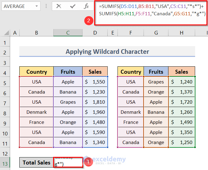
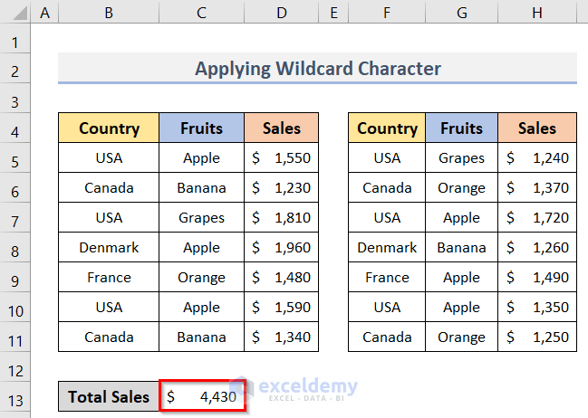
- Press the Enter key to get the result (see the screenshot below).
How Does the Formula Work?
- SUMIFS(D5:D11,B5:B11,”USA”,C5:C11,”*s*”): Adds the Sales for the USA with the Fruits containing ‘s’.
- SUMIFS(H5:H11,F5:F11,”Canada”,G5:G11,”*g*”): Sums up the Sales.
- Canada with the fruits containing ‘g’.
- SUMIFS(D5:D11,B5:B11,”USA”,C5:C11,”*s*”)+SUMIFS(H5:H11,F5:F11,”Canada”,G5:G11,”*g*”): Returns the summation of the two values gained from the two SUMIFS formula.
Download Practice Workbook
Download the practice workbook from here.
Related Articles
- SUMIFS with INDEX-MATCH Formula Including Multiple Criteria
- Excel SUMIFS Not Equal to Multiple Criteria
- [Fixed]: SUMIFS Not Working with Multiple Criteria
<< Go Back to Excel SUMIFS with Multiple Criteria | Excel SUMIFS Function | Excel Functions | Learn Excel
Get FREE Advanced Excel Exercises with Solutions!
