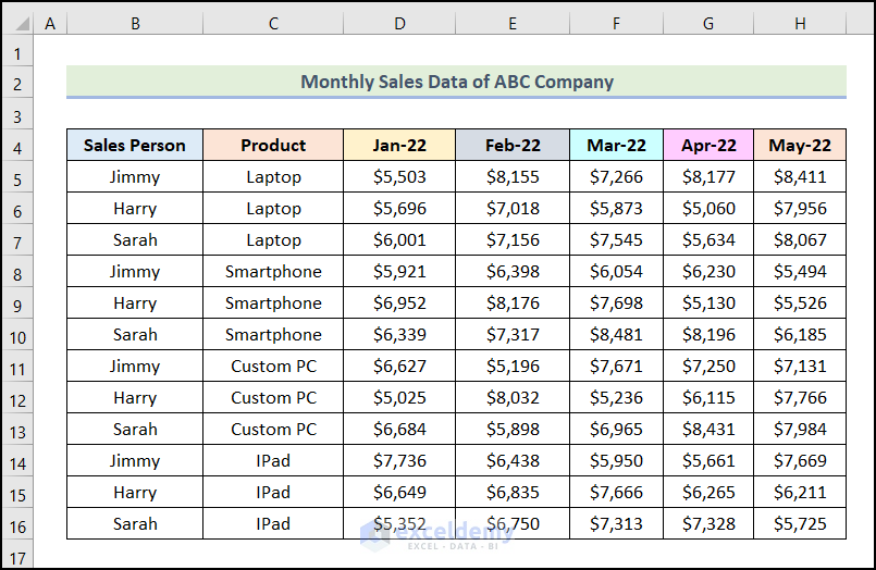
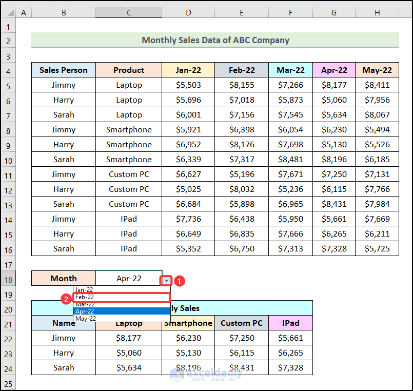
How to Apply the SUMIFS with the INDEX MATCH Functions to Multiple Columns and Rows

The dataset showcases the Monthly Sales Data of the ABC Company for various Products and for 3 Sales Persons. You want to find the Sales of a Sales Person based on the Month and Product.

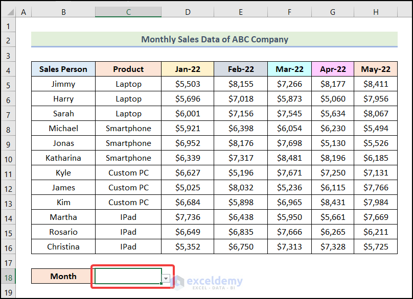
Step 1 – Creating a Drop-Down List to Select the Month

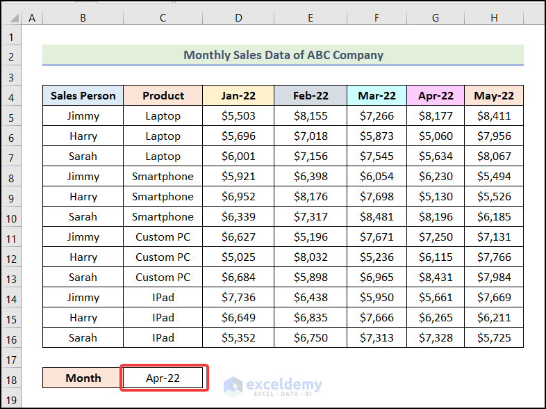
Create a cell named Month.

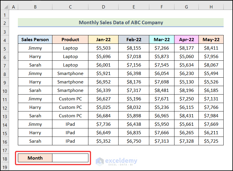
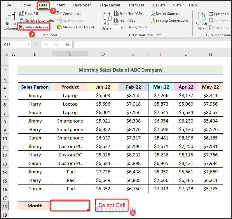
Select the cell beside Month. Here, C18.
Go to the Data tab.
Choose Data Validation in Data Tools.

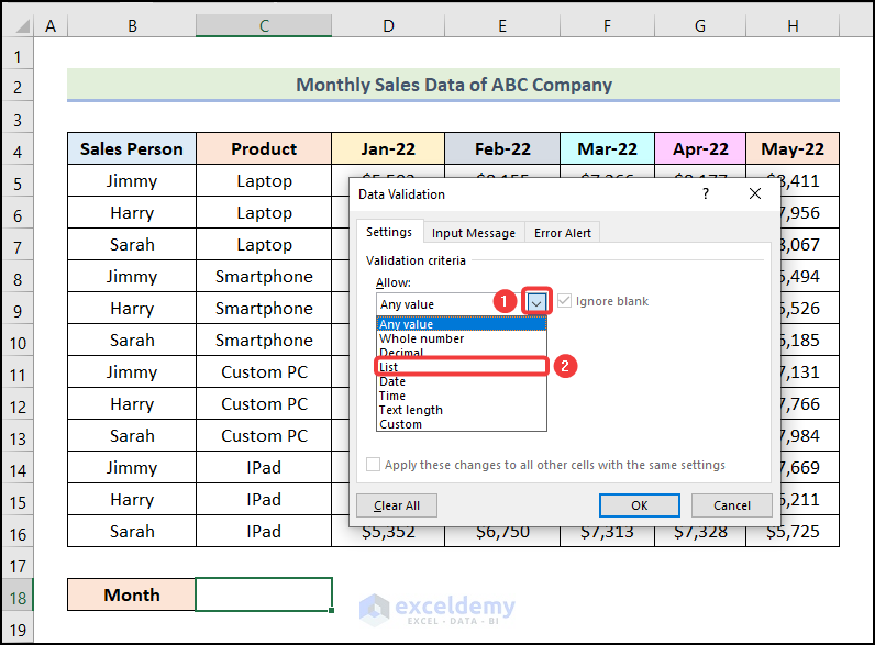
The Data Validation dialog box will open.

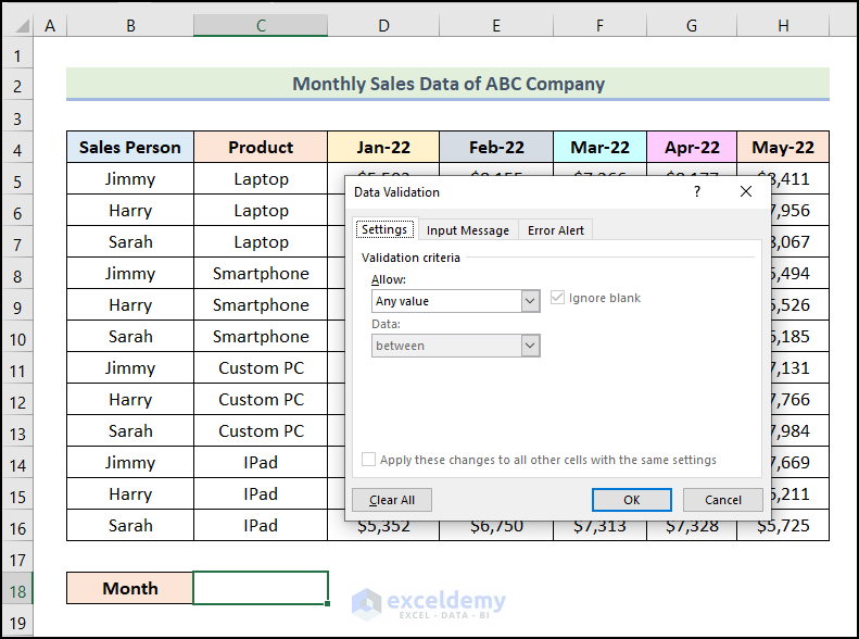
Click the drop-down icon.
Choose List.

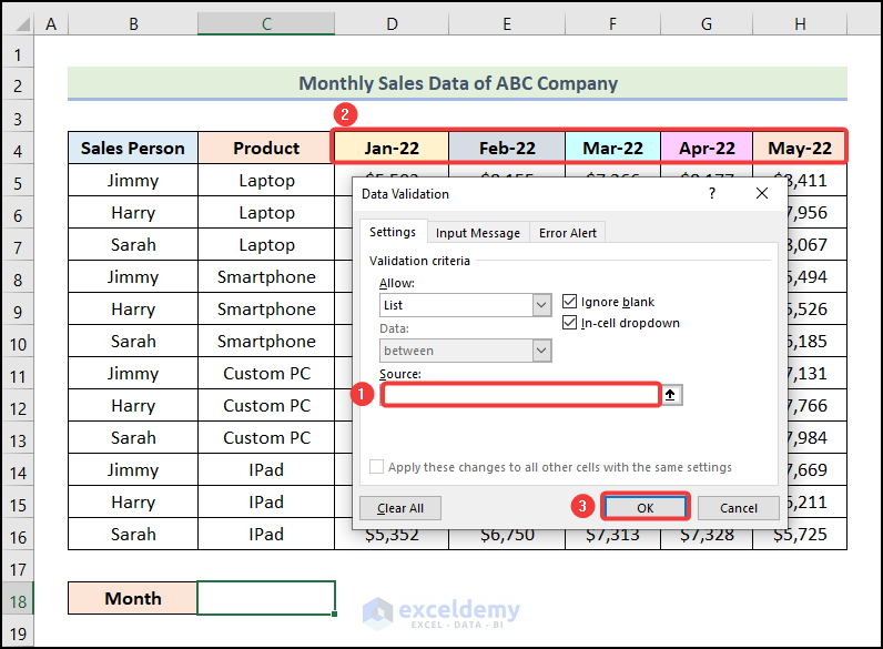
Click Source.
Select the range $D$4:$H$4.

$D$4:$H$4, indicates the names of the Months.

Click OK.

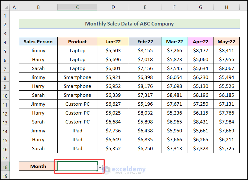
A drop-down icon will be displayed in C18.

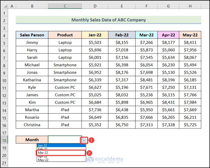
Step 2 – Checking the Drop-Down Button

Click the drop-down icon beside C18.
The name of the Months will be displayed in the drop-down. Choose Apr-22 (April-2022).

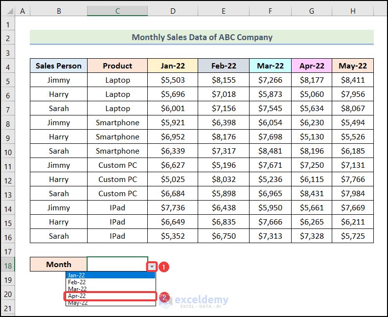
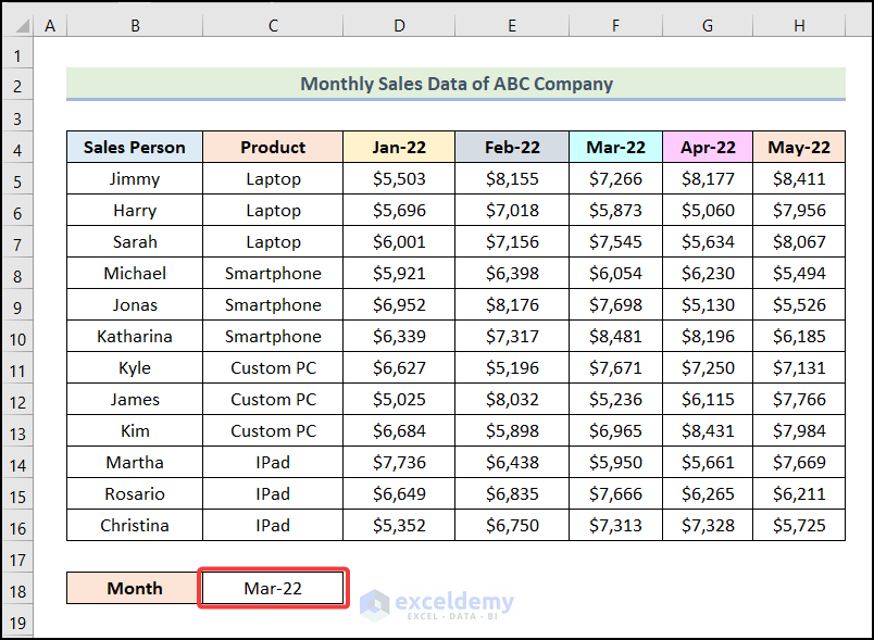
The name of the Month will be displayed in C18.

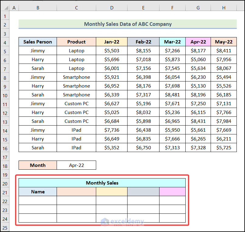
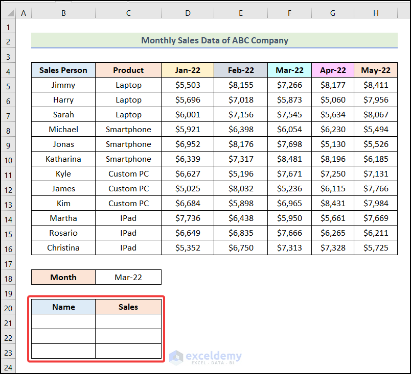
Step 3 – Creating an Output Table

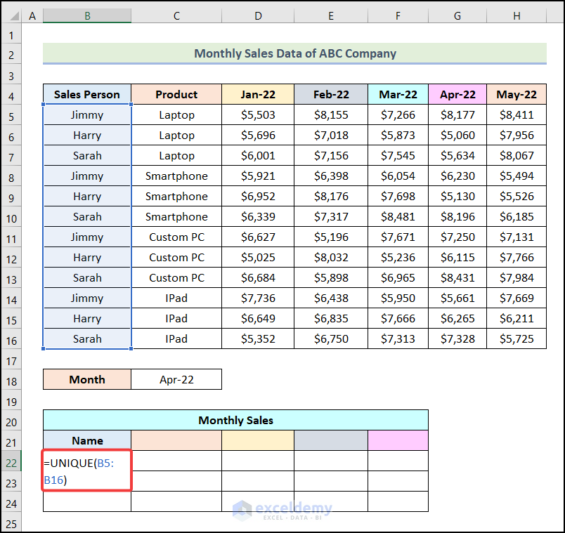
Create a table.

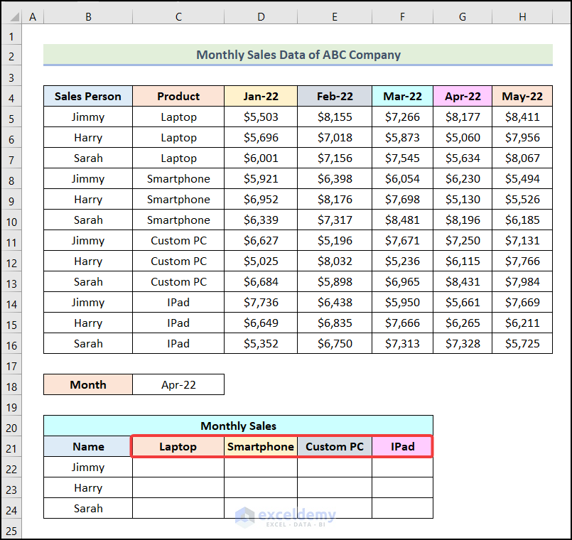
Enter the following formula in B22.

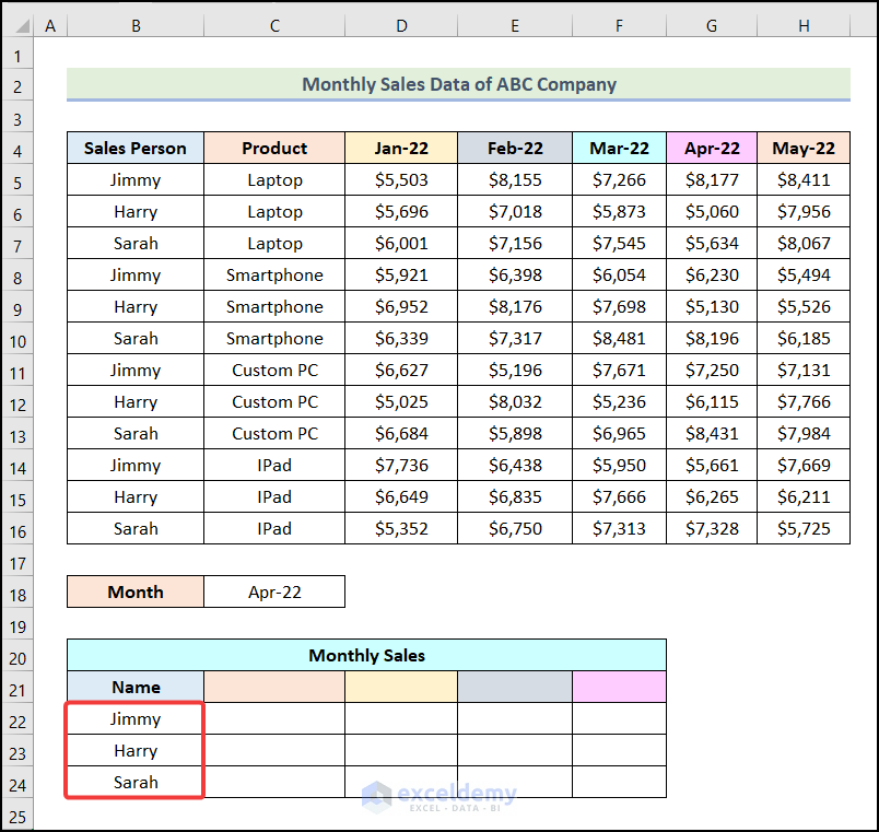
=UNIQUE(B5:B16)

B5:B16 refers to the cells of the Sales Person column.

Press ENTER.

You will see unique names from the Sales Person column.

Use the formula below in C21.

=TRANSPOSE(UNIQUE(C5:C16))

C5:C16 represents the cells in the Product column.

Press ENTER.

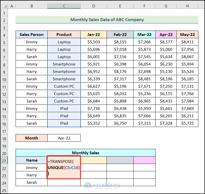
You will see the unique names of the Products in rows.

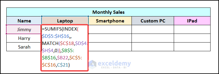
Step 4 – Using the SUMIFS Function with the INDEX-MATCH Functions

Enter the following formula in C22.

=SUMIFS(INDEX($D$5:$H$16,,MATCH($C$18,$D$4:$H$4,0)),$B$5:$B$16,$B22,$C$5:$C$16,C$21)

$D$5:$H$16 refers to Sales data for various Months; $C$18 indicates the selected Month; $D$4:$H$4 represents the array of all Months; $B22 indicates the Name of the Sales Person, and C$21 refers to the cell of the selected Product.

Formula Breakdown

MATCH($C$18,$D$4:$H$4,0) → gives the relative position of data in an array that matches a specific value.
- $C$18 → is the lookup_value argument.
- $D$4:$H$4 → is the lookup_array argument.
- 0 → indicates the [match_type] argument.
- Output → 4
INDEX($D$5:$H$16,,MATCH($C$18,$D$4:$H$4,0)) → It becomes INDEX($D$5:$H$16,,4)
- $D$5:$H$16 → refers to the array argument.
- 4 → is the column_num argument.
- Output → {8177;5060;5634;6230;5130;8196;7250;6115;8431;5661;6265;7328}.
SUMIFS(INDEX($D$5:$H$16,,MATCH($C$18,$D$4:$H$4,0)),$B$5:$B$16,$B22,$C$5:$C$16,C$21) → becomes SUMIFS({8177;5060;5634;6230;5130;8196;7250;6115;8431;5661;6265;7328},$B$5:$B$16,$B22,$C$5:$C$16,C$21)
- {8177;5060;5634;6230;5130;8196;7250;6115;8431;5661;6265;7328} → represents the sum_range argument.
- $B$5:$B$16 → is the criteria_range1 argument.
- $B22 → refers to the criteria1 argument.
- $C$5:$C$16 → is the criteria_range2 argument.
- C$21 → indicates the criteria2 argument.
- Output → $8,177

Press ENTER.

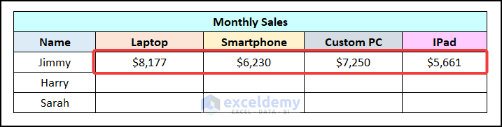
This is the output.

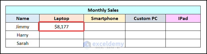
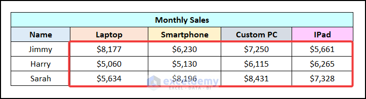
Drag the Fill Handle to F22 to see the Sales for Jimmy in Apr-22.

Use the AutoFill to see the Sales for Harry and Sarah.

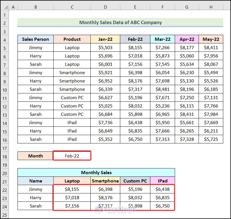
Step 5 – Checking if the Output is dynamic.

Click the drop-down icon beside C18.
Choose a month other than Apr-22 (April-2022). Here, Feb-22 (Februrary-2022).

The output will change automatically.

How to Use the SUMPRODUCT with INDEX and MATCH Functions in Excel

Steps:

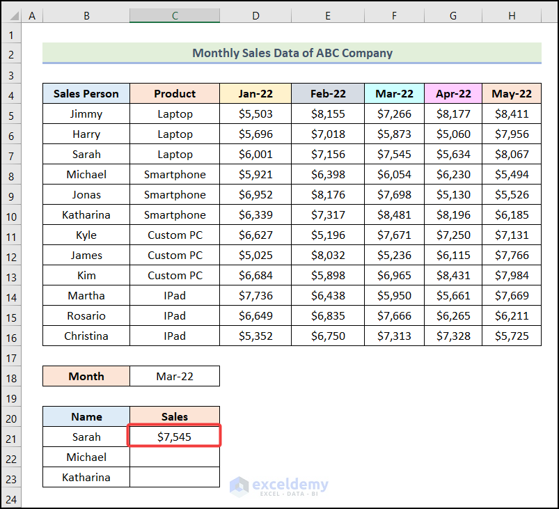
Follow the steps mentioned in Step 1 of method 1 to enable the drop-down icon beside C18.

Select a Month from the drop-down list. Here, March.

This is the output.

Create a table.

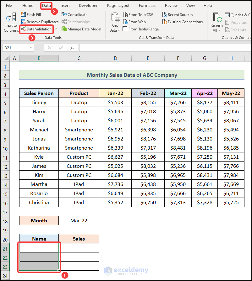
Select the cells under Name.
Go to the Data tab.
Choose Data Validation in Data Tools.

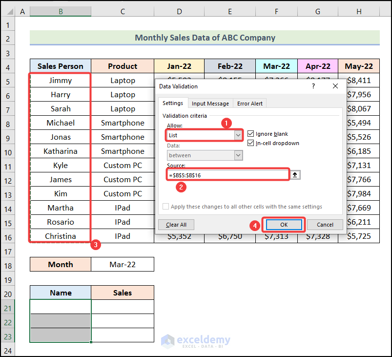
In the Data Validation dialog box, choose List.
Click Source.
Select the cells in the Sales Person column.
Click OK.

A drop-down icon will be displayed beside the Name column.

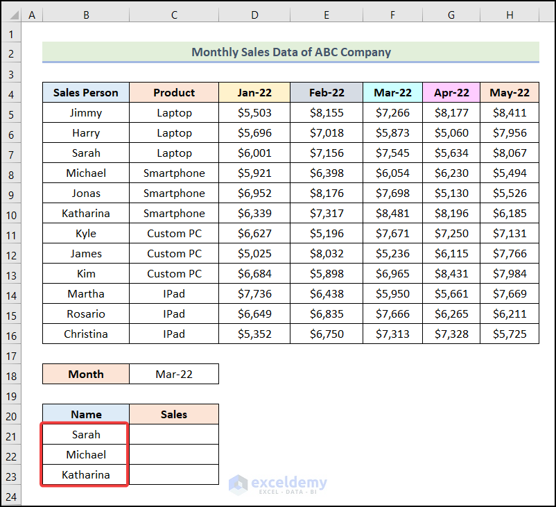
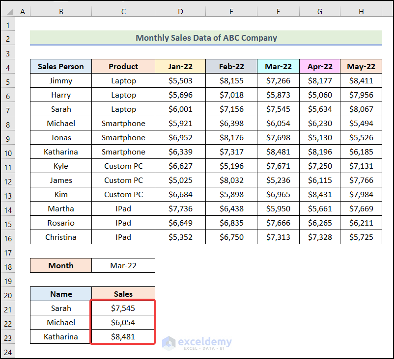
Click it and choose a Name. Here, Sarah.

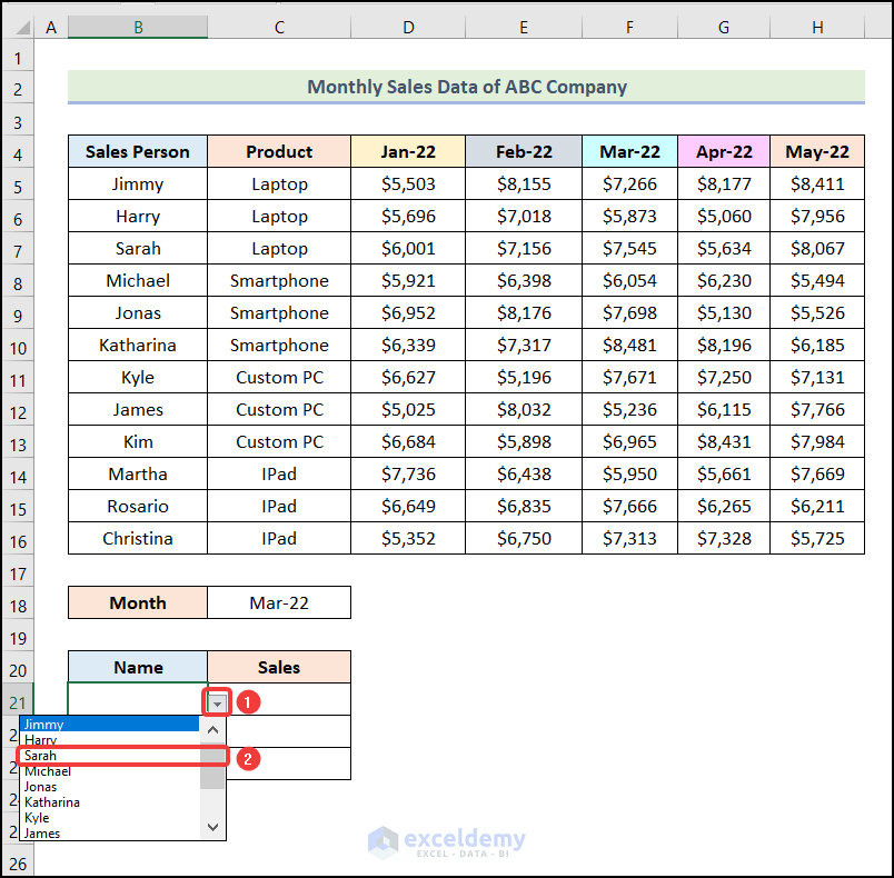
Choose 2 other names.

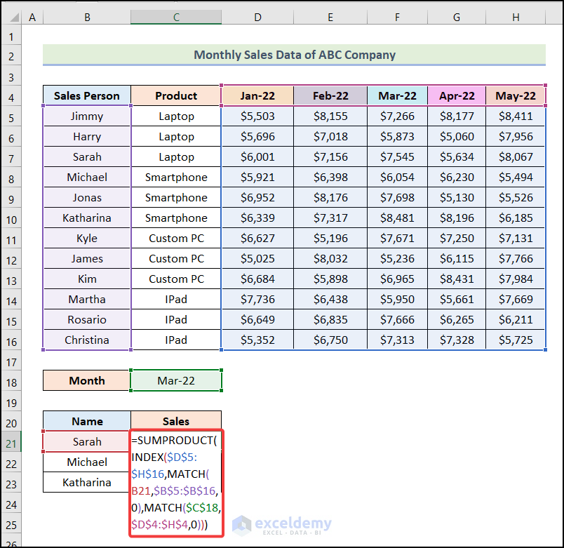
Enter the following formula in C21.

=SUMPRODUCT(INDEX($D$5:$H$16,MATCH(B21,$B$5:$B$16,0),MATCH($C$18,$D$4:$H$4,0)))

B21 refers to the cell in the Name column.

Formula Breakdown

MATCH(B21,$B$5:$B$16,0) → gives the relative position of data in an array that matches a specific value.
- B21 → is the lookup_value argument.
- $B$5:$B$16 → represents the lookup_array argument.
- 0 → is the [match_type] argument.
- Output → 3.
MATCH($C$18,$D$4:$H$4,0) → Output → 4.
INDEX($D$5:$H$16,MATCH(B21,$B$5:$B$16,0),MATCH($C$18,$D$4:$H$4,0)) → becomes INDEX($D$5:$H$16,3,4).
- $D$5:$H$16 → is the array argument.
- 3 → indicates the row_num argument.
- 4 → refers to the [column_num] argument.
- Output → 5634.
SUMPRODUCT(INDEX($D$5:$H$16,MATCH(B21,$B$5:$B$16,0),MATCH($C$18,$D$4:$H$4,0))) → becomes SUMPRODUCT(5634).
- Output → $5,634.

Press ENTER.

This is the output.

Use the AutoFill.

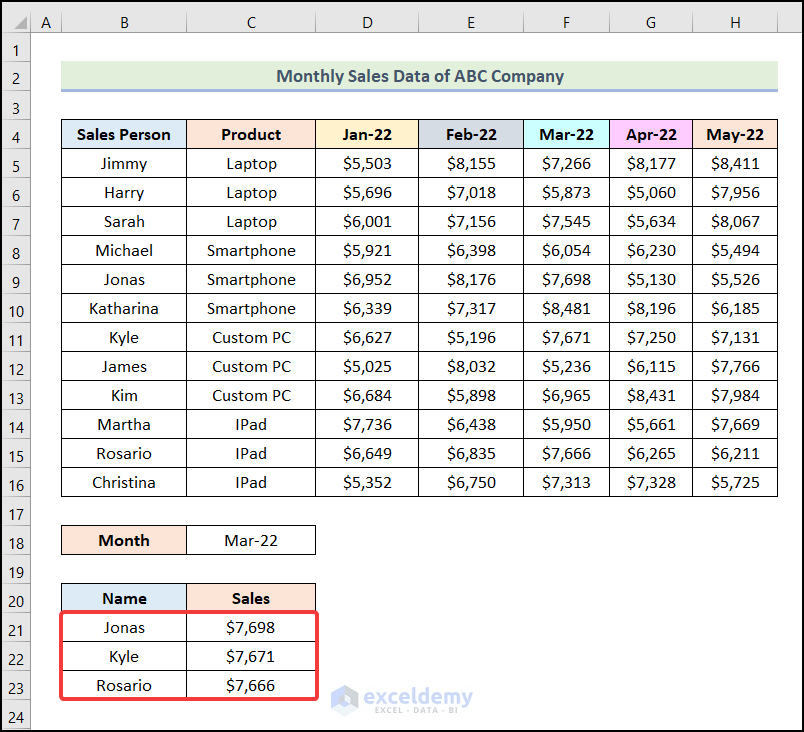
If you change the Name, the output will change.

You can also use the SUMPRODUCT function and a combination of INDEX and MATCH functions for multiple rows and columns.

Practice Section

Practice here.

Download Practice Workbook

SUMIFS with INDEX-MATCH Functions.xlsx

<< Go Back to Excel SUMIFS with Multiple Criteria | Excel SUMIFS Function | Excel Functions | Learn Excel

Get FREE Advanced Excel Exercises with Solutions!

4 Comments

Yosh Jul 25, 2023 at 1:02 AM

Can I incorporate the total number of YTD? Suppose the total YTD for only of June
- Reply
  Mahfuza Anika Era Jul 25, 2023 at 12:51 PM
  
  Dear Yosh,
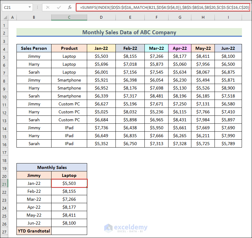
  Thank you for your query. Yes, you can determine the sum of YTD number. Firstly create a table like the following for each Month’s Sales of “Jimmy” for “Laptop”.
  Copy this formula in cell C21.
  =SUMIFS(INDEX($D$5:$I$16,,MATCH(B21,$D$4:$I$4,0)),$B$5:$B$16,$B$20,$C$5:$C$16,C$20)
  
  You will get the sales for each month.
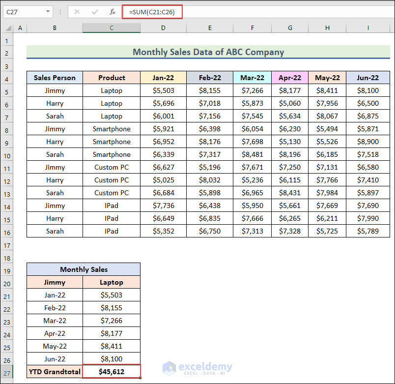
  Next, to calculate the “YTD Grandtotal” copy this formula in cell C27.
  =SUM(C21:C26)
  
  I hope this method will solve your problem. Thank you!
  Mahfuza Anika Era
  ExcelDemy
Yosh Jul 25, 2023 at 1:11 AM

If I want to calculate the subtotal of YTD? For example, the total YTD of Jimmy for laptop as of May
- Reply
  Mahfuza Anika Era Jul 25, 2023 at 12:13 PM
  
  Dear Yosh,
  I assume, this question is same as the previous one. You can follow the steps I have given in the previous reply. If you still have any confusion, please leave a comment describing your problem. Thank you!
  Mahfuza Anika Era
  ExcelDemy