Solving Transportation or Distribution Problems Using Excel Solver (2 Suitable Cases)

In this article, we will discuss 2 cases for solving transportation or distribution problems using the Excel Solver. It is well known that companies manufacture products at different locations and ship their products to customers at various locations. Distribution managers need to allocate and ship merchandise in the most efficient and cost-effective manner. This kind of problem is called the Transportation problem. Today, we will discuss 2 cases. Using these cases, you can easily use Solver for transportation or distribution problems in Excel.

Solving Transportation or Distribution Problems Using Excel Solver: 2 Suitable Cases

Today, we will discuss two cases of solving transportation or distribution problems using Excel Solver. In Case 1, we will try to minimize the total shipping cost while meeting requirements. And in Case 2, we will maximize after-tax profit with limited production capacity. You can see a quick view of Case 1 below.

Case 1: Minimize Total Shipping Cost While Meeting Requirements

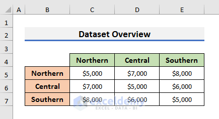
In the first case, we will try to minimize the total shipping cost while meeting all requirements using Solver in Excel. For that purpose, we need to understand the problem first. Suppose that northern, central, and southern California each uses 100 billion gallons of water each day. Also, assume that northern California and central California have 120 billion gallons of water available, whereas southern California has 60 billion gallons of water available. The cost of shipping 1 billion gallons of water between the three regions is as follows:

We need to find the cheapest way to deliver the amount of water each region needs.

Our objective, in this case, is to compute the total shipping cost and minimize it. The total cost can be expressed as follows:

(Number of billion gallons of water sent from Northern to Northern)*(Cost per billion gallons of sending water from Northern to Northern) + (Number of billion gallons of water sent from Northern to Central)*(Cost per billion gallons of sending water from Northern to Central) + (Number of billion gallons of water sent from Northern to Southern)*(Cost per billion gallons of sending water from Northern to Southern) + …… + (Number of billion gallons of water sent from Southern to Central)*(Cost per billion gallons of sending water from Southern to Central) + (Number of billion gallons of water sent from Southern to Southern)*(Cost per billion gallons of sending water from Southern to Southern)

If we translate the above model into an Excel formula, it will not only cost us a lot of time but also expose us to a high risk of making a mistake. So, let’s follow the steps to see how we can implement an easier formula and use Solver to find the minimum shipping cost.

STEPS:

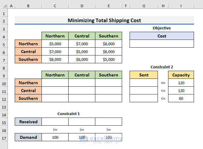
First of all, we need to create a dataset to enter the shipments for each supply point to each region.
Here, the range C10:E12 depicts that. These are the “By Changing Cells” that we will use inside the Solver tool.

Secondly, we need to assign cells for the Objective and Constraints.
In our case, Cell G5 is the Objective cell that will hold the minimum shipping cost.
Similarly, range C15:D17 represents Constraint 1 and range G10:I12 denotes Constraint 2.
Constraint 1 says the Demand for water in each region should be equal to or greater than 100 gallons. After minimizing, we will get the Received amount of water in the range C12:C14.
On the other hand, Constraint 2 denotes that northern and central California have the capacity of water equal to or less than 120 gallons whereas southern California has the capacity equal to or less than 60 gallons of water. After minimizing, we will get the gallons of water in the range G10:G12 that should be SENT.

In the following step, we need to type the formula below in Cell G5 to get the Total Shipping Cost:

=SUMPRODUCT(C5:E7,C10:E12)

In this formula, we have used the SUMPRODUCT function. In order to find the total cost, we put the costs of shipping 1 billion gallons of water between those three regions in cell range C5:E7. Shipments for each supply point to each region were put in cell range C10:E12. These two ranges are of the same dimensions and therefore SUMPRODUCT function can be used to compute the total cost here.

So far, we have determined our Objective and the “By Changing Cells”.
Now, we need to apply equations for the constraints.
As Constraint 2 states that water sent from each region must be equal to or less than the gallons of water available, we can use the formula below in Cell G10 to compute the total gallons of water sent from Northern California:

=SUM(C10:E10)

Drag down the Fill Handle up to Cell G12 to get the amount of water sent from Central and Southern California.

Here, we have used the SUM function to find the resultant of the range C10:E10.

On the other hand, Constraint 1 is that water received by each region should be equal to or greater than 100 billion gallons of water.
This constraint was put in the range C15:E17 and the formula below is used to count the Received amount in Cell C15:

=SUM(C$10:C$12)

Now, drag the Fill Handle to the right up to Cell E15 to copy the formula.

After inserting the formulas, go to the Data tab and select Solver from the Analyze section. It will open the Solver Parameters box.

Fill the dialog box as shown in the below figure.
Total Shipping Cost is computed by adding together the terms changing cell*constant in Cell G5. So, “Set Objective” is G5.
After that, select Min and type range C10:E12 in the “By Changing Variable Cells” field.
Two explicit constraints are created by comparing sums of changing cells with a constant. We have inserted the constraints using the Add option.
You can see that both our objective and constraints can be represented by a linear relationship. Therefore, our model is a linear model, and the Simplex LP engine was selected.
Obviously, shipments must be positive and that’s the reason why we selected the Make Unconstrained Variables Non-Negative check box.
After that, click on the SOLVE option.

Again, click OK in the Solver Results box.

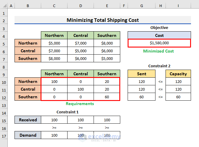
Finally, you will find the requirements and total shipping cost automatically.

The minimum cost of meeting requirements is $1,580,000 and we can achieve it by applying the following schedule:

We can send 100 billion gallons of water from Northern to Northern and 20 billion gallons of water from Northern to Southern.
Also, we can transfer 100 billion gallons of water from Central to Central and 20 billion gallons of water from Central to Southern.
Southern keeps all available water for its own use.

Case 2: Maximize After-Tax Profit with Limited Production Capacity

In the second case, we will minimize the after-tax profit with limited production capacity with the Solver add-in. To illustrate the example, we will use the problem below:

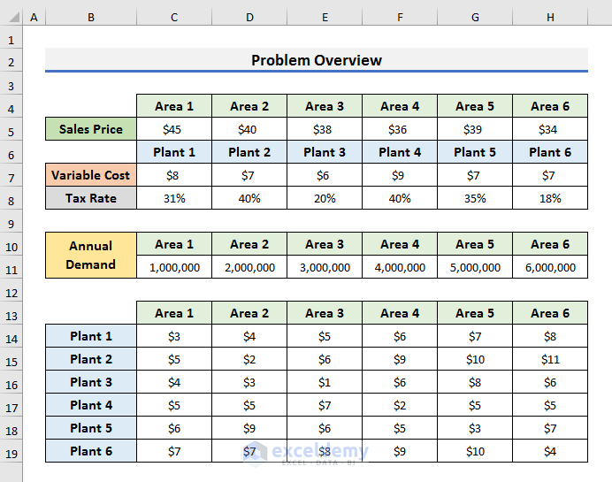
A company produces and sells drugs at several locations. The decision of where to produce goods for each sales location can have a huge impact on profitability. Suppose that we need to produce drugs at six plants and sell them to customers in six areas. The “tax rate” and “variable production cost” depend on the place of production. The “sales price” of each drug depends on the selling place. Also, each of the six plants can produce up to 6 million units per year. You can see the annual demand for the products in each area in the problem overview below. The unit shipping cost depends on the plant and area. You can find the details in the overview below.

We need to find the maximum after-tax profit with the limited production capacity.

Let’s follow the steps below to see how we maximize the profit using the Solver tool in Excel.

STEPS:

Firstly, we need to create a dataset for computation.
Since tax rate, variable production cost, and sales price relate to the location of production or sale, we can simplify the problem by computing profit for each plant and then adding them together.
You can see the rearranged dataset with the Profit column. Here, we will count the profit for each plant.

Secondly, insert cells for “By Changing Variable Cells” in the range C14:H19. These cells will contain the number of drags sent from Plants to the Areas.
Also, one constraint states that the capacity of the plants is less than 6 million units. We insert that constraint in the range J4:L19.

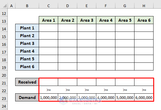
Again, the second constraint denotes the amount of the Received and Demand units. It is in the range C21:H23 like the picture below.

Now, to compute the after-tax Profit, type the formula below in Cell K5:

=(SUMPRODUCT(C14:H14,$C$11:$H$11)-J14*I5-SUMPRODUCT(C14:H14,C5:H5))*J5

Press Enter and drag down the Fill Handle up to Cell K10.
Then, in Cell K11, type the formula below:

=SUM(K5:K10)

After that, type the formula below in Cell J14 to count the number of drugs sent from plants to locations:

=SUM(C14:H14)

Hit Enter and drag the Fill Handle down to Cell J19.

To find the Received number of drugs, type the formula below in Cell C21:

=SUM(C14:C19)

Press Enter and drag the Fill Handle to the right to Cell H21.

In the following step, navigate to the Data tab and select Solver from the Analyze section. It will open the Solver Parameters box.

In the Solver Parameters box, fill the dialog box as shown in the below figure.
Here, we computed the Total Profit by adding the profit of each plant. So, “Set Objective” is K11.
After that, select Max and type range C14:H19 in the “By Changing Variable Cells” field.
Now, insert the constraints using the Add option.
The first constraint is that each location should receive drugs equal to or greater than the demands. We can describe it using “$C$21:$H$21 >= $C$23:$H$23“.
Another constraint is that the produced drugs cannot be greater than the capacity. You can write it using “$J$14:$J$19 <= $L$14:$L$19”.
You can see that both our objective and constraints can have a linear relationship. Therefore, our model is a linear model, we will use Excel Solver for Linear Programming and we need to select the Simplex LP engine.
Obviously, shipments must be positive and that’s the reason why we selected the Make Unconstrained Variables Non-Negative check box.
After that, click on the SOLVE option.

Again, click OK to proceed.

As a result, you will see the maximum profit amount in Cell K11.

Also, you will get the number of drugs that you need to send to locations using constraints in the range C14:H19.

Here, all six plants should produce 6 million units of drugs to get a maximum profit of $332,630,000.

Download Practice Workbook

You can download the practice workbook from here.

Solving Transportation Problem.xlsx

Conclusion

In this article, we have demonstrated 2 cases of Solving Transportation or Distribution Problems Using Excel Solver. I hope this article will help you to perform your tasks efficiently. Furthermore, we have also added the practice book at the beginning of the article. To test your skills, you can download it to exercise. Lastly, if you have any suggestions or queries, feel free to ask in the comment section below.

<< Go Back to Excel Solver Examples | Solver in Excel | Learn Excel

Get FREE Advanced Excel Exercises with Solutions!

Solving Transportation or Distribution Problems Using Excel Solver (2 Suitable Cases)

Solving Transportation or Distribution Problems Using Excel Solver: 2 Suitable Cases

Case 1: Minimize Total Shipping Cost While Meeting Requirements

Case 2: Maximize After-Tax Profit with Limited Production Capacity

Conclusion

Related Articles

Leave a reply Cancel reply