Create a Resource Allocation Model in Excel – 5 Steps

What Is a Resource Allocation Model in Excel?

A resource allocation model involves:

• Identifying the skill sets needed to finish project tasks.
• Calculating how long these tasks will take in hours.
• Planning the resource capacity, which entails choosing who will work on what tasks based on availability predictions and the project schedule.

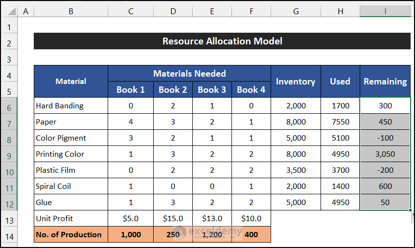
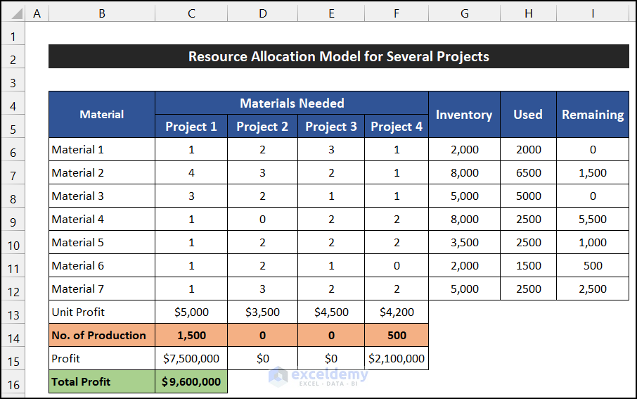
Consider the production process of four books.

This is an overview:

Step 1- Entering Data

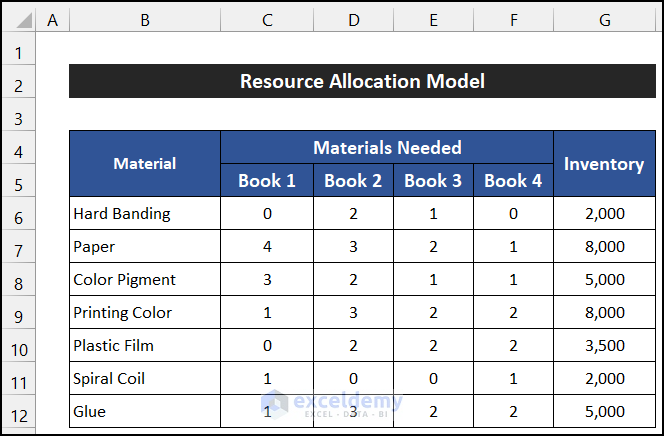
• Create a dataset in B4:F14. Enter project names row-wise and the materials list column-wise.

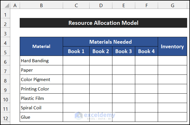
• Enter all necessary data.

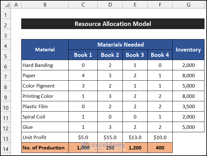
• Allot two rows to define the Unit Profit and Number of Productions.
• Enter the amount for each book.

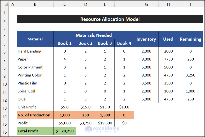
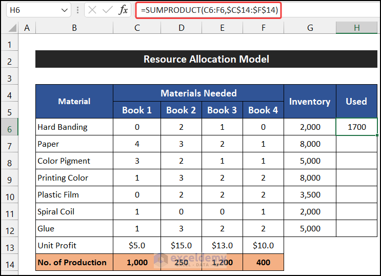
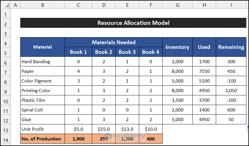
Step 2 – Estimating the Amounts of the Used Inventory

• Select H6.
• Enter the following formula using the SUMPRODUCT function to get the used amount of the material. Use an Absolute Cell Reference in C14:F14.

• Press Enter.

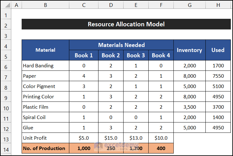
• Drag down the Fill Handle to copy the formula to the other cells.

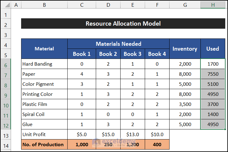
• You will see the amounts of inventories used during the production.

Step 3 – Calculating the Remaining Inventory

• Select I5.
• Enter the following formula in the cell.

• Press Enter.

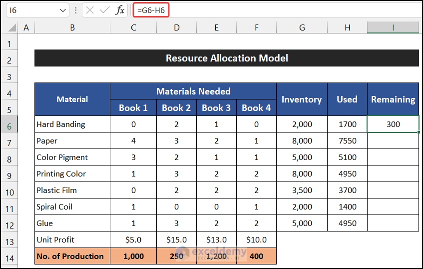
• Drag down the Fill Handle to copy the formula to the other cells.

• You will see the result.

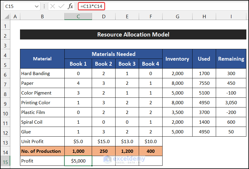
Step 4 – Evaluating the Profit

• Define B15 as Profit to see the profit of a book.
• Select C15 and enter the following formula.

• Press Enter.

• Drag down the Fill Handle to copy the formula to the other cells.

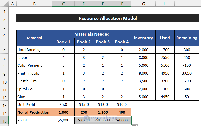
• To evaluate the total profit, define B16 as the Total Profit.
• Enter the following formula using the SUM function.

• Press Enter.

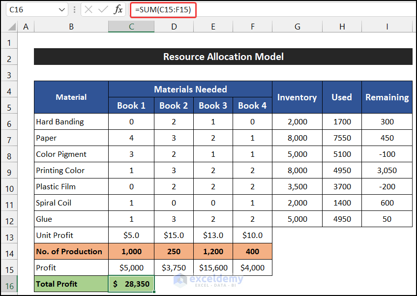
• You will see the total profit value.

Step 5 – Applying the Solver Analysis Toolpak for Maximum Profit

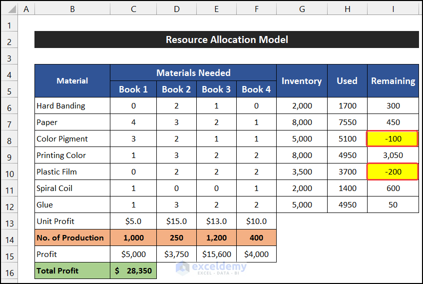
Some of the remaining inventory values are negative. Extra raw materials are needed for production.

Use the Solver ToolPak to check the maximum profit amount and the corresponding book amount.

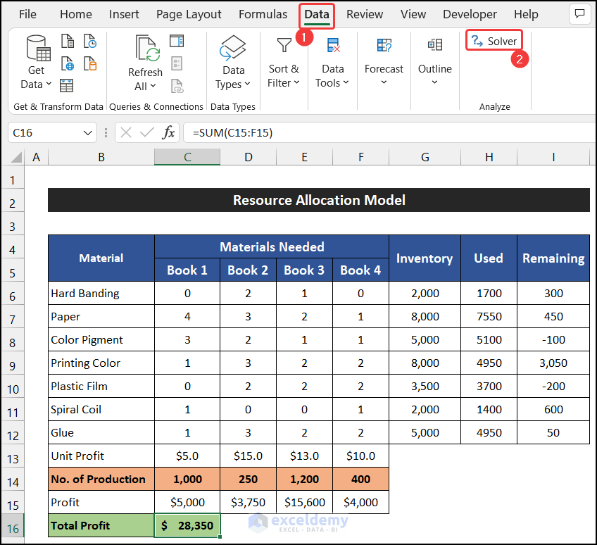
• Go to the Data tab and click Solver in Analysis. (You can enable it in Excel Options.)

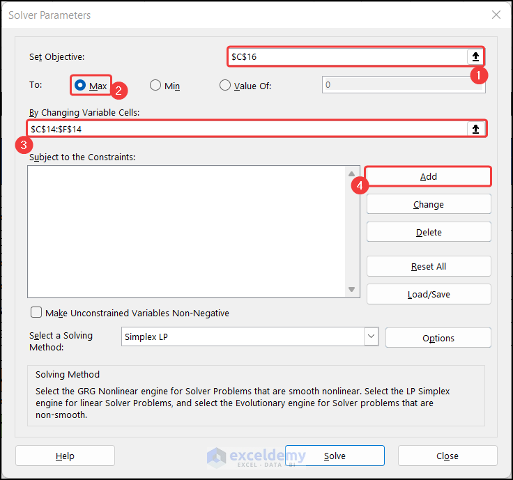
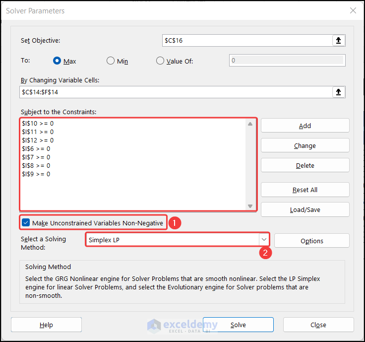
• In the Solver Parameters dialog box, in Set Objective, select cell C16.
• Choose Max.
• Define By Changing Variables Cells as C14:F14.
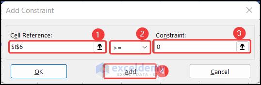
• Add constraints. Click Add.

• In Add Constraint, select I6 in Cell Reference.
• Change the condition operator ‘<=’ to ‘>=’.
• In Constraints, enter 0.
• Click Add.

• Add the same types of constraints to I7:I12.
• Click OK.
• You will see all constraints in the empty list box.
• Check Make Unconstrained Variables Non-Negative.
• Set Select a Solving Method to Simplex LP.
• Click Solve.

• The value of C14:F14 will change. The Solver tool-pak will display Solver Result.
• Click OK to keep the value.

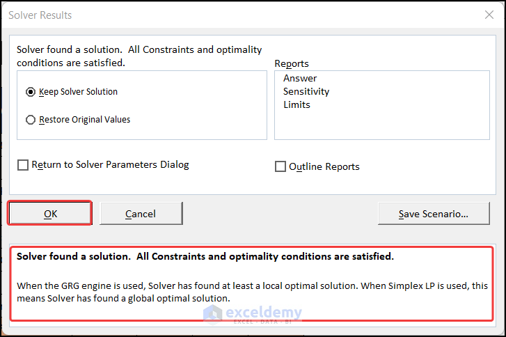
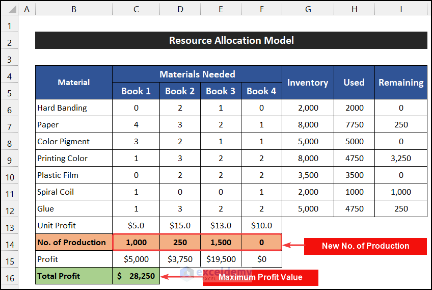
• The value of maximum profit and the amount of production of each book to secure the profit are displayed.

How to Do Resource Allocation for a Project

Define the project name row-wise. Enter the names of raw materials in the columns. This is the output

Read More: How to Do Portfolio Optimization Using Excel Solver

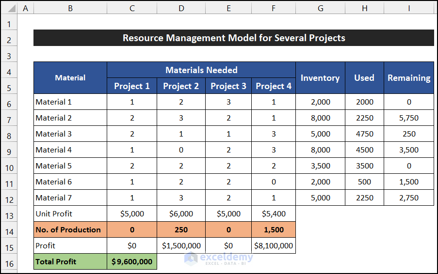
How to Do Resource Management in Excel Sheet

To create a completely new management model, you can follow the procedure of the resource allocation model.

Read More: How to Use Excel Solver for Linear Programming

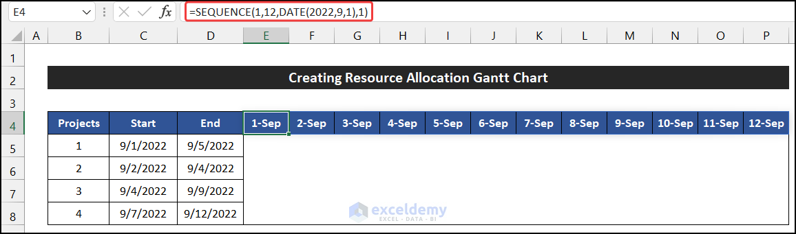
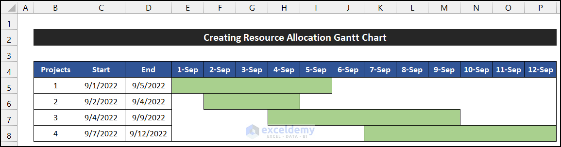
How to Create a Resource Allocation Gantt Chart in Excel

You can  add a Gantt chart to resource allocation to check the working period of the project. Use the Conditional Formatting feature.

 Steps:

• Enter the following formula in E4 to get the dates in  E4:P4 using the SEQUENCE function.

• Press Enter.

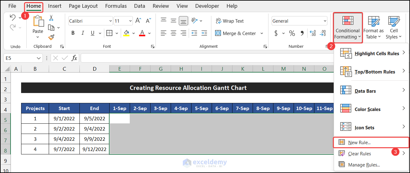
• Select E5:P8.
• In the Home tab, click the drop-down arrow of Conditional Formatting in Styles.
• Select New Rule.

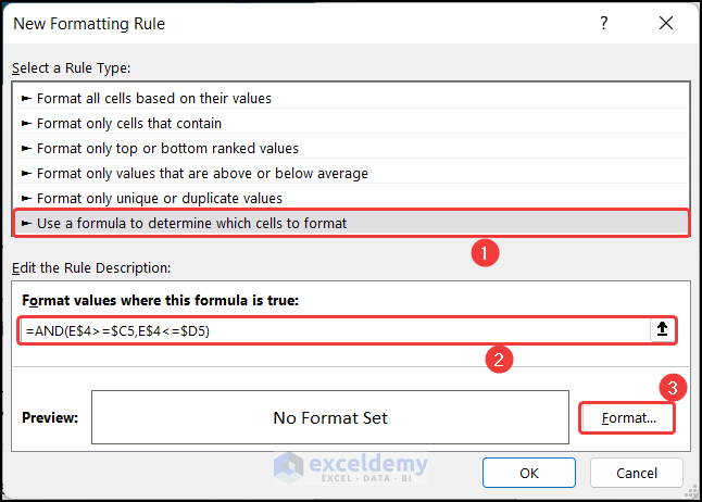
• In New Formatting Rule, choose Use a formula to determine which cells to format.
• Enter the following formula with the AND function.

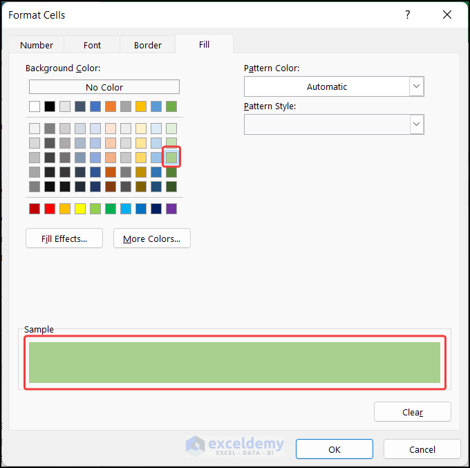
• Click Format.

• In Format Cells, in the Fill tab, choose a background color. Here, Green, Accent 6, Lighter 60%.
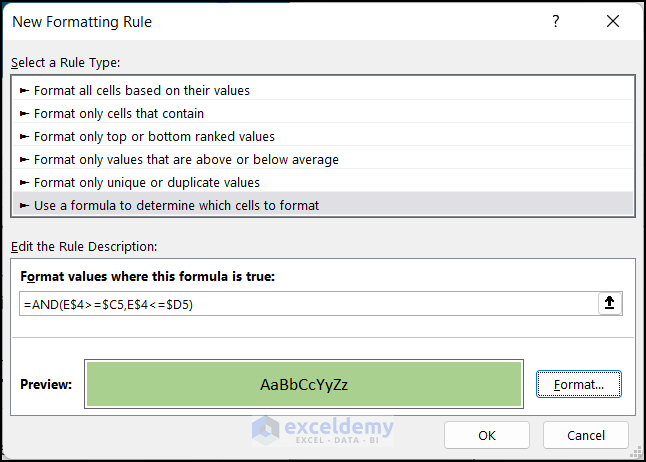
• Click OK to close the Format Cells dialog box.

• Click OK to close the New Formatting Rule dialog box.

• The chart will be displayed.

Read More: Example with Excel Solver to Minimize Cost

Download Practice Workbook

Download the practice workbook.

Related Articles

• How to Use Excel Solver to Rate Sports Team
• How to Use Excel Solver to Determine Which Projects Should Be Undertaken?
• Solving Sequencing Problems Using Excel Solver Solution
• Solving Transportation or Distribution Problems Using Excel Solver
• How to Assign Work Using Evolutionary Solver in Excel
• Solving Equations in Excel

<< Go Back to Excel Solver Examples | Solver in Excel | Learn Excel