Example with Excel Solver to Minimize Cost

What Is the Solver in Excel?

Solver is a Microsoft Excel add-in program. The Solver is part of the What-If Analysis tools that we can use in Excel to test different scenarios. It can solve decision-making issues by finding the optimal values. The Solver can also analyze how changing values impacts the worksheet’s output.

How to Add the Solver to Excel

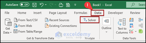
You can access Solver by choosing the Data tab, then going to Analyze and selecting Solver. You may have to install the Solver add-in:

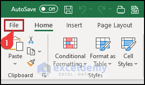
Choose the File tab.

Select Options from the menu.

The Excel Options dialog box appears.
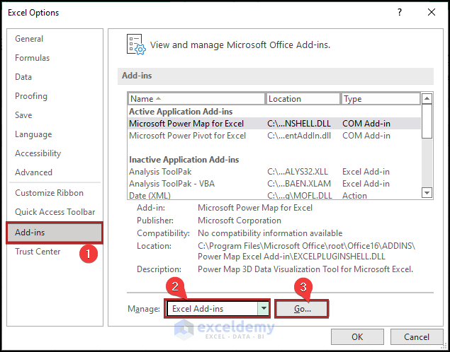
Go to the Add-Ins tab.
At the bottom of the Excel Options dialog box, select Excel Add-Ins from the Manage drop-down list and then click Go.

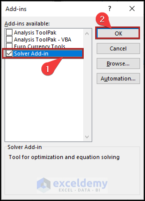
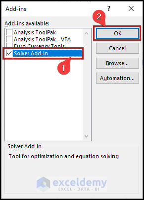
The Add-ins dialog box appears.
Check the Solver Add-In and click OK.

We can also install the Solver add-in using the Developer tab. Just follow along.

Go to the Developer tab.
Click on Excel Add-ins on the Add-ins group.

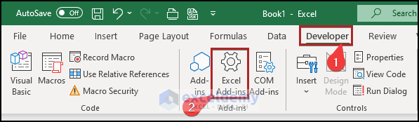
This opens the Add-ins wizard.
Enable Solver.

Once you activate the add-ins in your Excel workbook, they will be visible on the ribbon.
Go to the Data tab.
You can find the Solver add-in in the Analyze group.

How to Use the Solver in Excel

Set up the worksheet with values and formulas. Make sure that you have formatted cells correctly; for example, the maximum time you can’t produce partial units of your products, so format those cells to contain numbers with no decimal values.
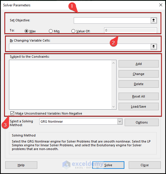
Open the Solver. The Solver Parameters dialog box will appear.
Specify the target cell. The target cell also is known as the objective.
Specify the range that contains the changing cells.
Specify the constraints.
Change the Solver options if needed.
Let the Solver solve the problem.

Introduction to Solver Parameters

The Excel Solver determines the best solution based on the objective cell formula.

here are the common values used in the Solver Parameters dialog box:

Objective Cell: The cell with a formula we want to test based on its independent variables.

Variable Cells: Variable data that the Solver modifies during testing.

Constraint Cells: Constraints that the solution must adhere to or the prerequisites that must be met.

Using the Excel Solver to Minimize Cost

Example 1 – Minimize Shipping Cost

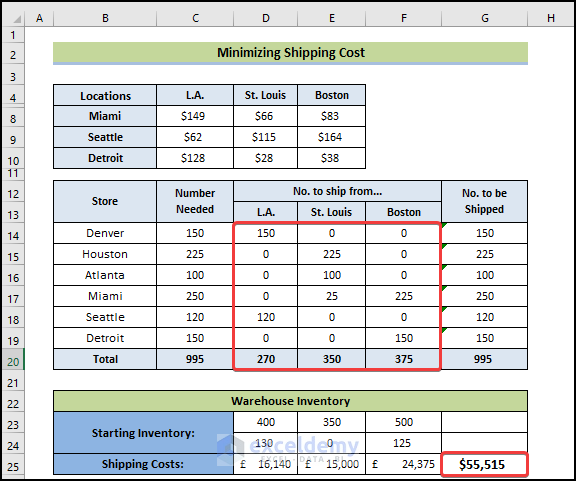
We have a dataset that contains various warehouses and stores, as well as shipping prices per unit between every location and store. Given the limited supply in each warehouse, we have to supply each store with enough inventory while minimizing the shipping costs.

Shipping Costs Table: This table contains the cell range B4:E10. This is a matrix that holds per-unit shipping costs from each warehouse to each retail outlet. For example, the cost to ship a unit from Boston to Detroit is $38.

Product needs of each retail store: This information appears in the cell range C14:C19. The retail outlet in Houston needs 225, Denver needs 150 units, Atlanta needs 100 units, and so on. C18 is a formula cell that calculates the total units needed from the outlets.

No. to ship from: These cell values will be varied by Solver.

Warehouse inventory: Row 21 contains the amount of inventory at each warehouse. For example, the Los Angeles warehouse has 400 units of inventory. Row 22 contains formulas that show the remaining inventory after shipping.

Calculated shipping costs: Row 24 contains formulas that calculate the shipping costs.

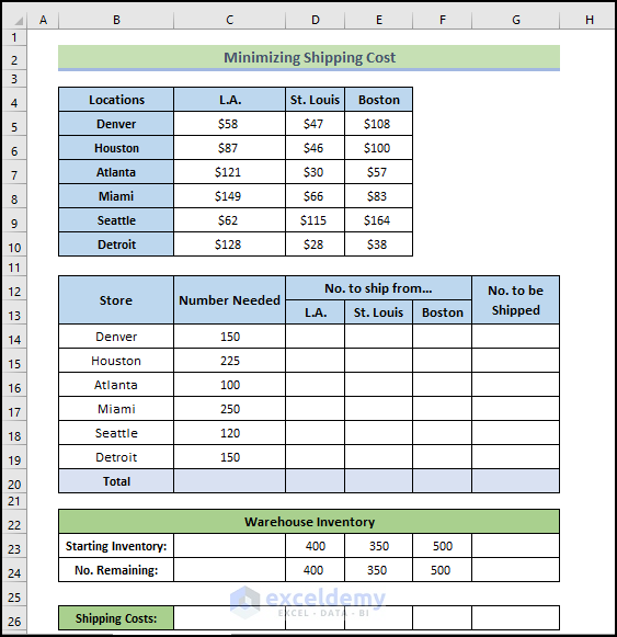
The solver will fill in the values in the cell range D14:F19 in such a way that will minimize the value in cell G24 by adjusting the values of cell range D14:F19 fulfilling the following constraints:

The number of units demanded by each retail outlet must equal the number shipped. In other words, all the orders will be filled:

C14=G14, C16=G16, C18=G18, C15=G15, C17=G17, and C19=G19

The number of units remaining in each warehouse’s inventory must not be negative: D24>=0, E24>=0, F24>=0.
The adjustable cells can’t be negative because shipping a negative number of units makes no sense. The Solve Parameters dialog box has a handy option: Make Unconstrained Variables Non-Negative.

Steps:

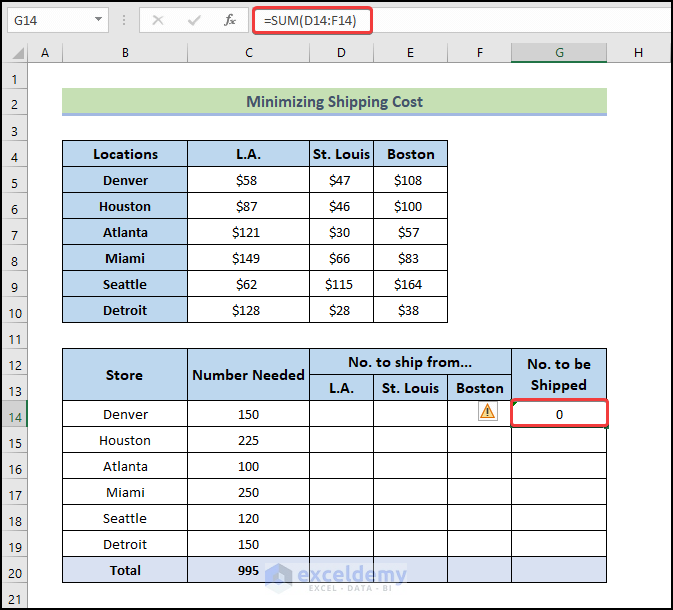
To calculate No. to be shipped, use the following formula.

=SUM(D14:F14)

Press Enter.

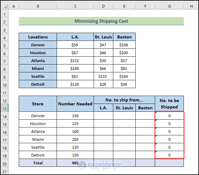
Dag the Fill Handle icon down to cell G19 to fill the other cells with the formula.

Use the following formula for the total.

=SUM(C14:C19)

Press Enter.

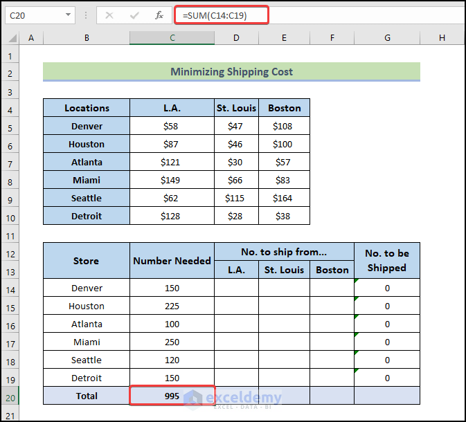
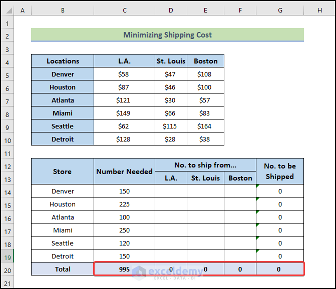
Drag the Fill Handle icon to the right to cell G20 to fill the other cells with the formula.

To calculate the shipping costs, use the following formula.

=SUMPRODUCT(C5:C10,D14:D19)

Press Enter.

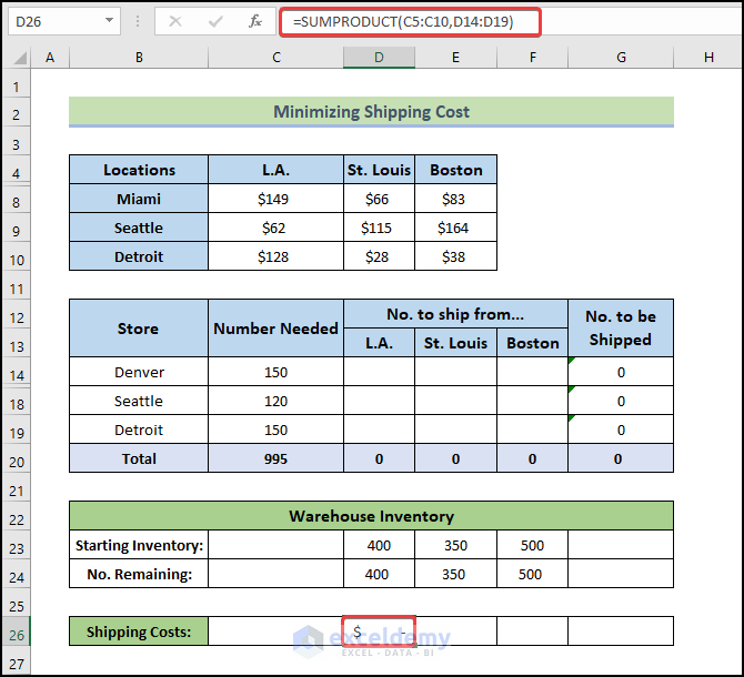
Drag the Fill Handle icon to the right up to cell F26 to fill the other cells with the formula.
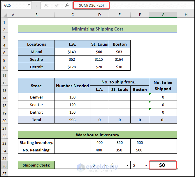
Use the following formula in cell G26.

=SUM(D26:F26)

Press Enter.

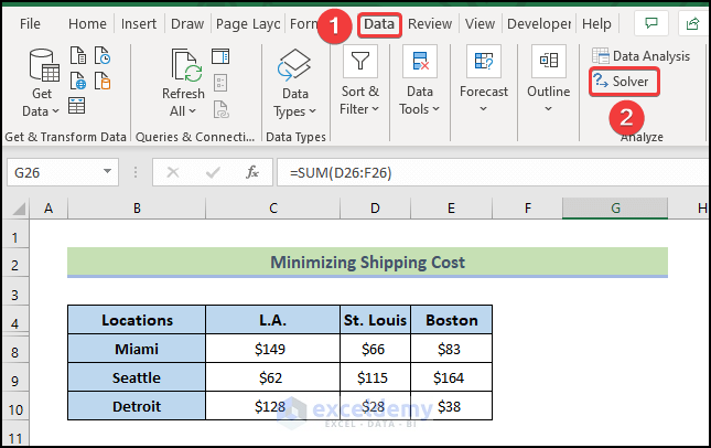
To open the Solver Add-in, go to the Data tab and click on Solver.

In the Set Objective field, insert $G$26.
Select the radio button of the Min option.
In the field By Changing Variable Cells put $D$14:$F$19 or select the range from the table (use the arrow icon on the box).
Add constraints: C14=G14, C16=G16, C18=G18, C15=G15, C17=G17, C19=G19, D24>=0, E24>=0, and F24>=0. These constraints will be shown in the Subject to the Constraints field.
Check the Make Unconstrained Variables Non-Negative box.
Select Simplex LP from the Select a Solving Method drop-down list.

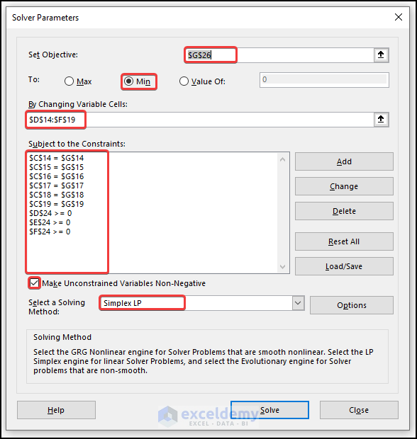
Click on the Solve button. The following figure shows the Solver Results dialog box. Once you click OK, your result will be displayed.

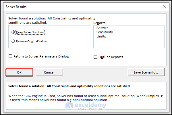
The Solver displays the solution shown in the following figure.

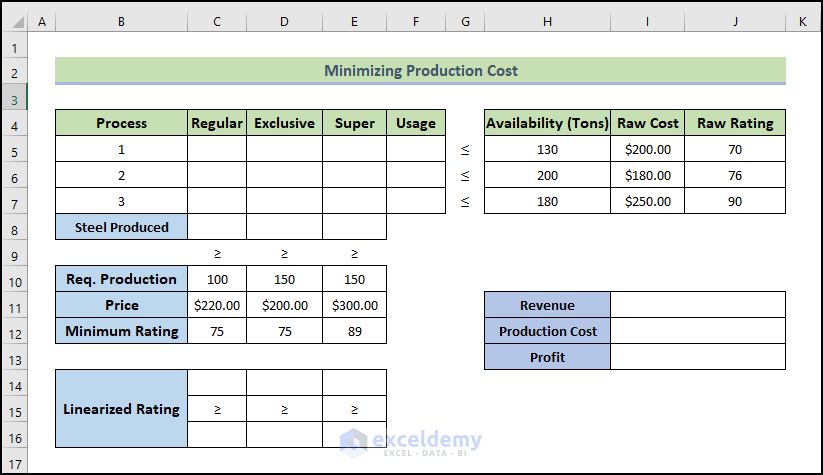
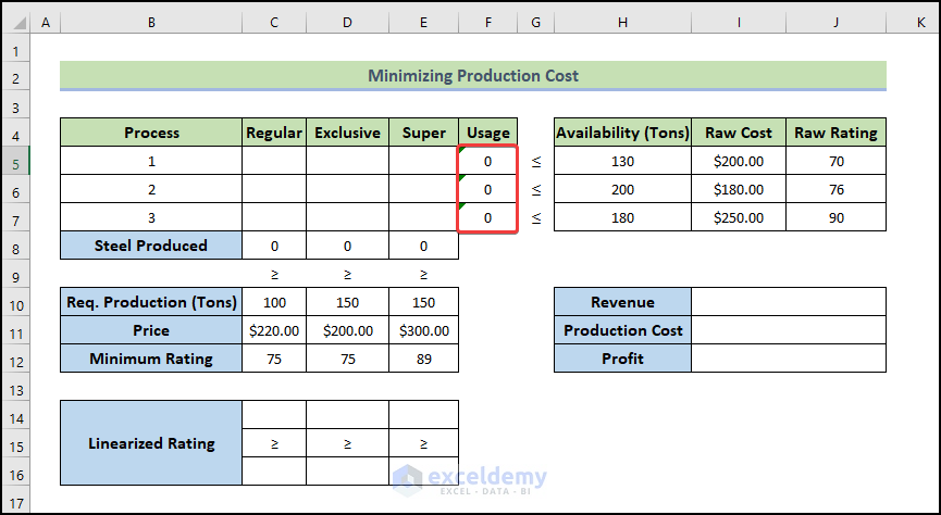
Example 2 – Minimize Production Cost

With the following dataset, we will mix different raw materials to produce different types of steel, such as regular, exclusive, and super-quality steel. We have data about the availability and cost of these raw materials, as well as their quality rating. We established the required amount of production, the price per ton of different classes of steel, and their minimum rating. We also have a parameter called the Linearized Rating.

Steps:

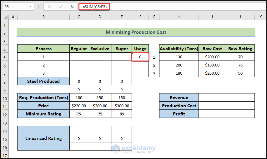
Use the following formula in cell F5.

=SUM(C5:E5)

The formula calculates the total amount of the type 1 Steel (Regular, Exclusive, and Super) that will be produced from the first available resources.

Press Enter.

Drag the Fill Handle icon to cell F7 to fill the other cells with the formula.

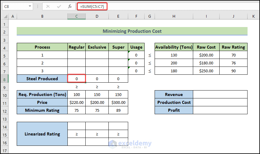
Use the following formula for the calculation of the total Regular Steel production amount.

=SUM(C5:C7)

Press Enter.
Drag the Fill Handle icon up to cell E8 to fill the other cells with the formula.

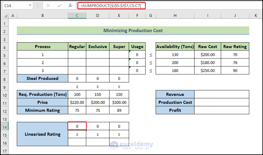
Use the formula below in cell C14 to calculate the Linearized Rating and fill the adjacent cells up to E14.

=SUMPRODUCT($J$5:$J$7,C5:C7)

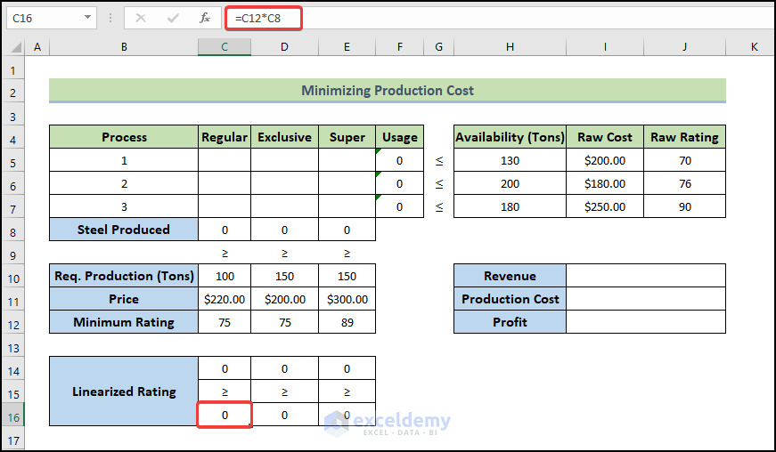
Use the following formula C16, and fill the cells up to E16.

=C12*C8

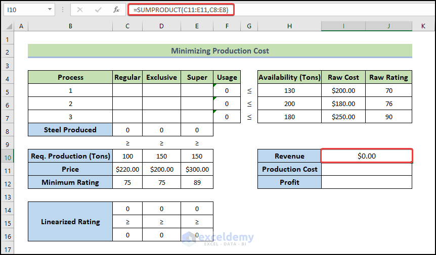
Use the formula below in cell I10 to determine the Revenue.

=SUMPRODUCT(C11:E11,C8:E8)

Press Enter.

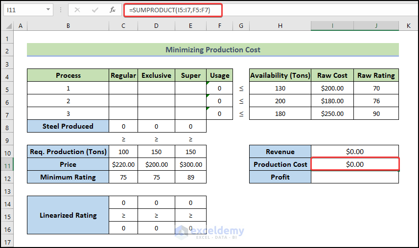
To calculate the production cost, use the following formula:

=SUMPRODUCT(I5:I7,F5:F7)

Press Enter.

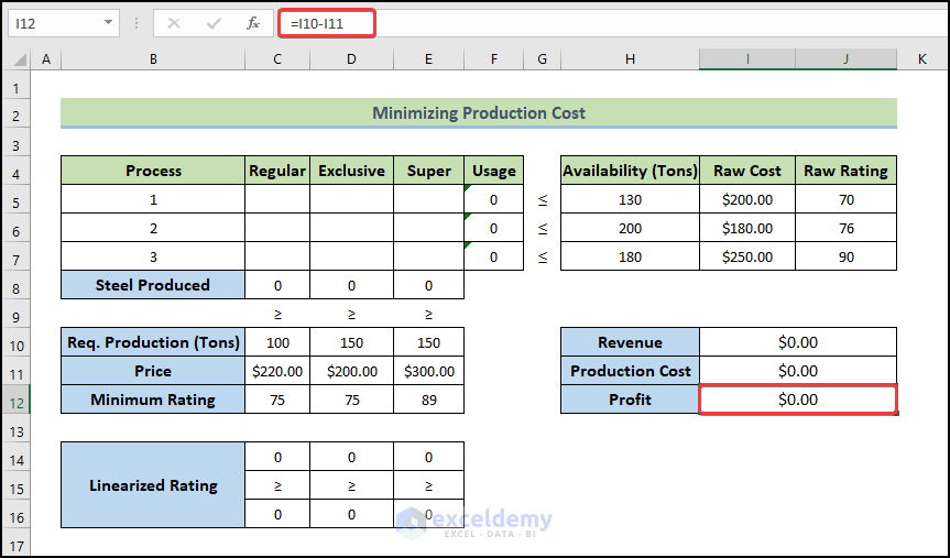
The following formula will return the Profit.

=I10-I11

Press Enter.

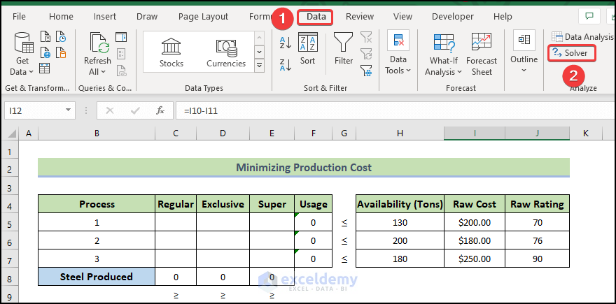
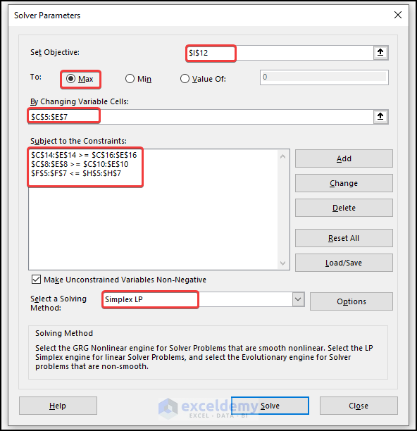
Go to the Data tab and click on Solver.

Enter the Subject, Changing Variables, and Constraints.
Set objective to I12.
Our changing variables are the Steel products, so this range will be C5:E7.
The Linearized Raw Rating needs to be greater than or equal to the Linearized Minimum Required Rating, so C14:E14>=C16:E16.
The production amount will be greater than the required amount: C8:E8>=C10:E10.
The usage of raw materials can’t exceed the available raw materials: F5:F7<=H5:H7.

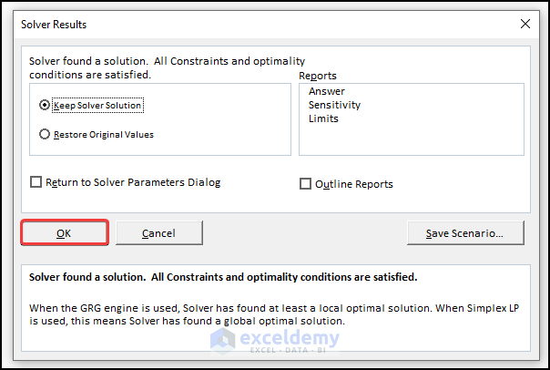
After clicking on Solve, you will get the following window. Click on OK.

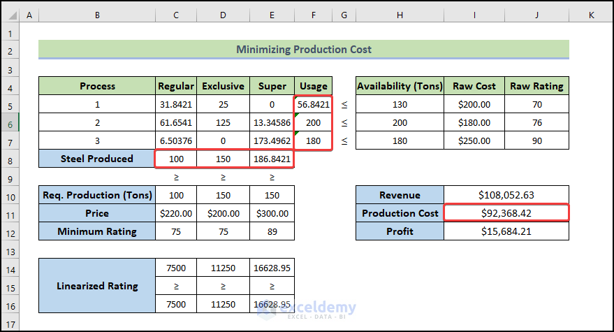
You will get the values of how much Raw Materials you should use to get the minimum production cost.
You will also get the optimized Revenue, Cost of production, and Profit.

Download the Practice Workbook

Minimize Cost.xlsx

<< Go Back to Excel Solver Examples | Solver in Excel | Learn Excel

Get FREE Advanced Excel Exercises with Solutions!

4 Comments

[email protected] Sep 15, 2016 at 9:09 AM

Cannot download example file. It keeps directing me to mailchimp and then I’m seeing error because I’m already subscribed.
- Reply
  Kawser Sep 15, 2016 at 11:21 AM
  
  Check your email please, Smith!
Ahmed Mar 4, 2021 at 8:26 AM

Hi,
I hope you can help me in that using excel

The Kellogg’s Cornflake Company began in 1906 with the Kellogg brothers who originally ran a sanatorium in Michigan, USA. They experimented with different ways to cook cereals without losing the goodness. Their philosophy was ‘improved diet leads to improved health’. Between 1938 and the present day Kellogg’s opened manufacturing plants in the UK, Canada, Australia, Latin America and Asia. Kellogg’s is now the world’s leading breakfast cereal manufacturer. Its products are manufactured in 3 countries; Belgium (location 50,4) with total capacity 25000 tons and distribution costs per unit 6$; China (location 39, 116) with total capacity 28000 tons and distribution costs per unit 9$; and France (location 48, 2) with total capacity 37000 tons and distribution costs per unit 5$, while sold in more than 3 countries; Greece (location 37, 23) with total demand 15000 tons and distribution costs per unit 9$; Ireland (location 53, 6) with total demand 18000 tons and distribution costs per unit 4$; and Luxembourg (location 49, 6) with total demand 28000 tons and distribution costs per unit 9$. It produces a wide range of cereal products, including the well-known brands of Kellogg’s Corn Flakes, Rice Krispies, Special K, Fruit n’ Fibre, as well as the Nutri-Grain cereal bars. Kellogg’s business strategy is clear and focused: • to grow the cereal business – there are now 40 different cereals • to expand the snack business – by diversifying into convenience foods • to engage in specific growth opportunities.

Questions
1. In order to minimize total distribution costs, design a facility location model to determine the right location of establishing a distribution center.
2. Design a distribution network and generate an answer report to determine the flow of goods between suppliers and markets.
3. Is it feasible to shut down one supply markets to minimize total costs if you know that the fixed costs are as follows: Belgium (18000 $), China (17000 $), and France (19000$)? Generate an answer report to shows your results.
- Reply
  Kawser Mar 5, 2021 at 10:47 PM
  
  Hi Ahmed,
  I am keeping a note of your problem, hope we shall be able to make a solution to this.
  Thanks.