In this article, we will demonstrate how to create a dependent drop down list in Excel. To explain the process, we’ll use the following data set with the Names, Authors, and Book Types of some books in a bookshop.

Our objective is to create a dependent drop-down list.
- First, we will create a drop-down list of the Book Types (First Drop Down List)
- Then we will create a drop-down list of the Authors based on the Book Types (Middle Drop Down List)
- Finally, we will create a drop-down list of the Book Names based on the Authors (Last Drop Down List)
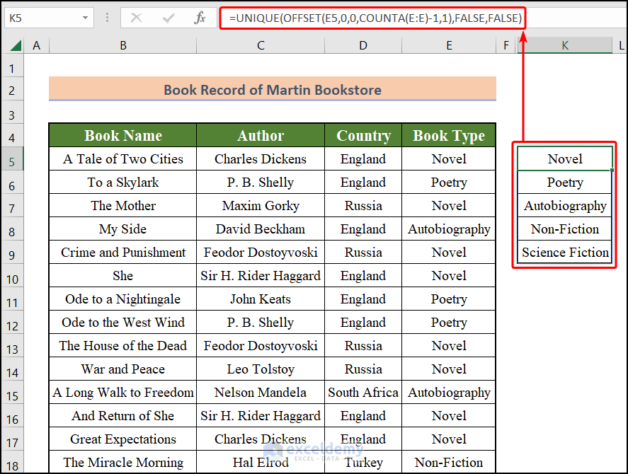
Step 1 – Create the First Drop Down List Using the UNIQUE Function
- Select any cell outside the dataset and apply the UNIQUE function as follows:
=UNIQUE(D5:D30,FALSE,FALSE)
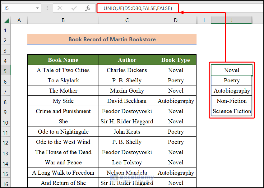
Here, D5:D30 is the range of the array (Book Type).
- Select the cell to enter the drop-down list.
- Go to Data > Data Validation > Data Validation.
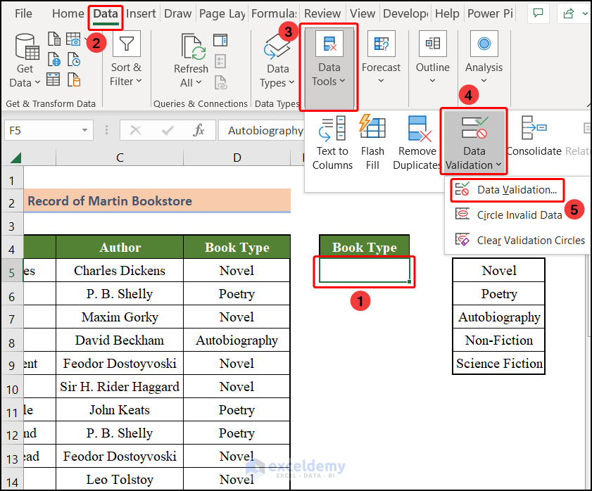
- Click on Data Validation.
The Data Validation dialog box will open.
- From the Allow option, select List.
- In the Source box, enter the absolute cell reference of the previously entered formula, with a HashTag (#) at the end. In this example, $J$5#
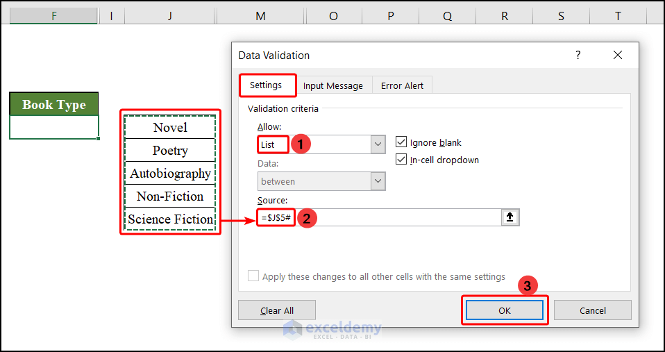
- Click on OK.
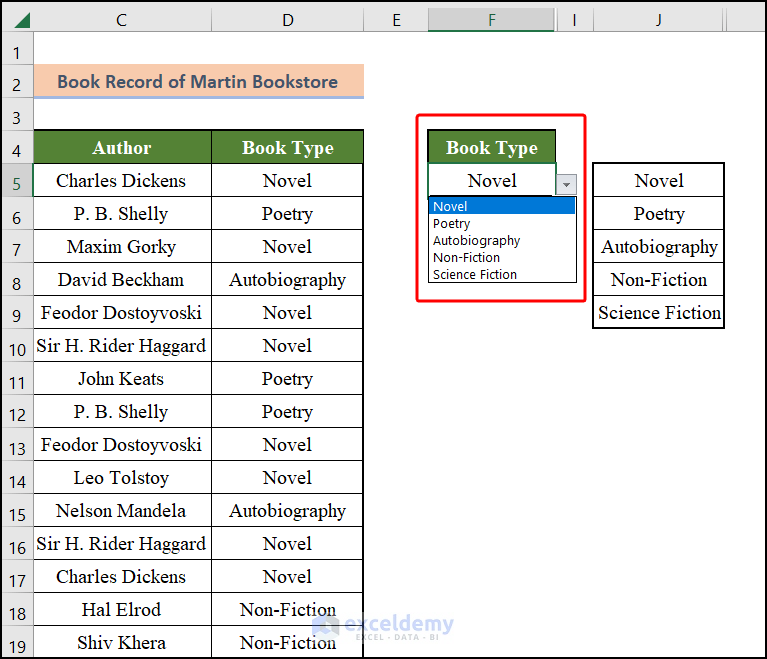
A drop-down list of the Book Types is generated in the selected cell.
Note:
- To generate a dynamic drop-down list, use this formula combining the UNIQUE, OFFSET and COUNTA functions instead:
=UNIQUE(OFFSET(E5,0,0,COUNTA(E:E)-1,1),FALSE,FALSE)
Here, we simply replace the column array D5:D30 with the OFFSET function, which takes this form:
=OFFSET(start_cell,0,0,COUNTA(column)-1,1)
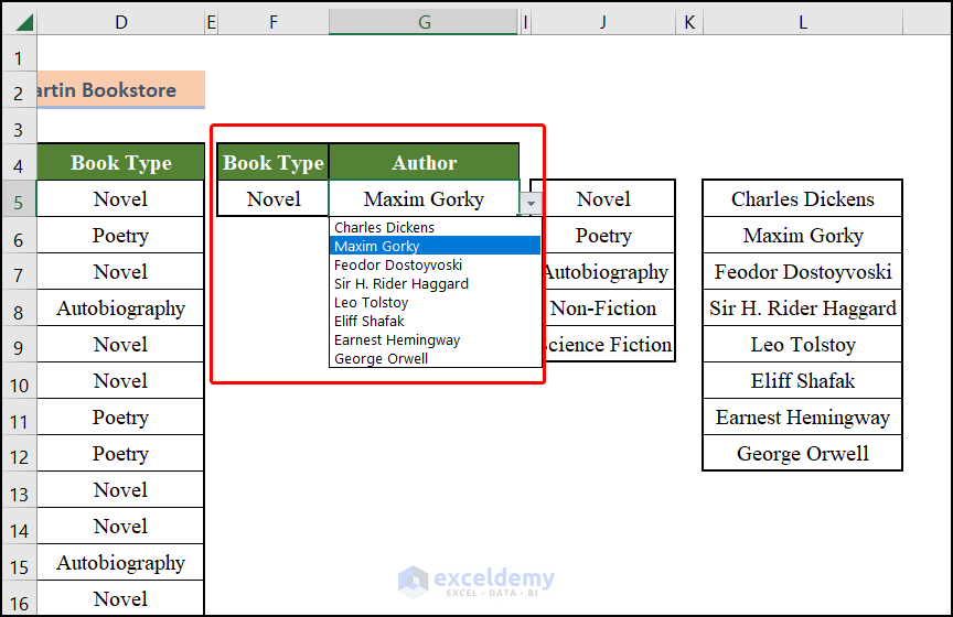
Step 2 – Create the Middle Drop Down List (First Dependent List) with the UNIQUE-FILTER Function Combination
Now we will create a drop-down list of the Authors based on the Book Type selected from the first list.
- Select any cell outside the dataset and enter this formula combining the UNIQUE and FILTER functions:
=UNIQUE(FILTER(C5:C30,E5:E30=G5),FALSE,FALSE)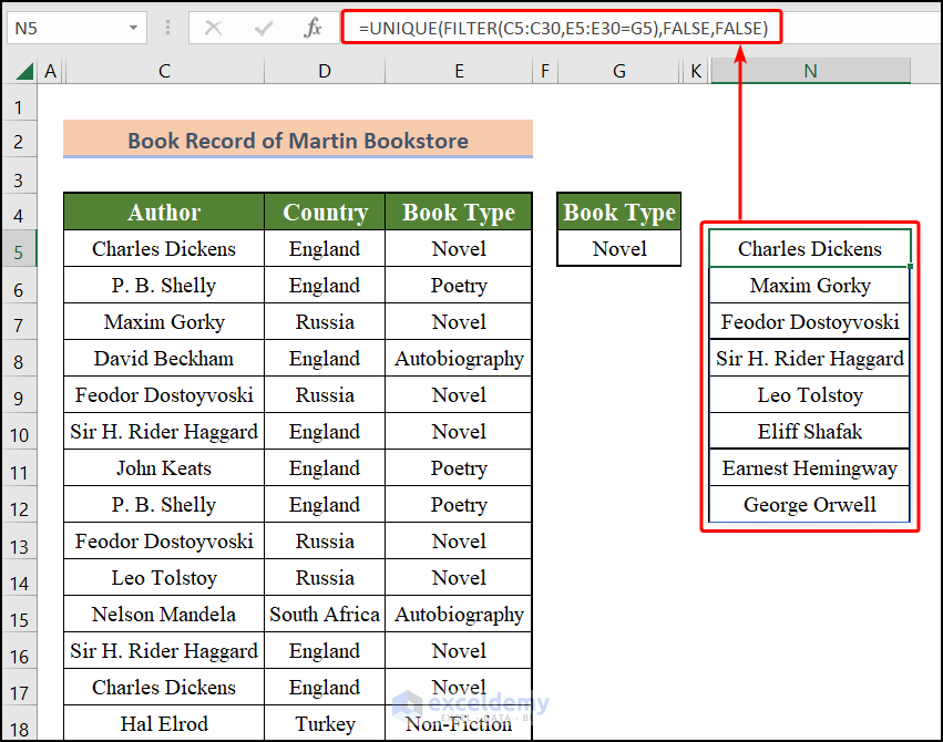
Here, C5:C30 is the range of this drop-down list (Authors), and D5:D30 is the range of the previous drop-down list (Book Types). F5 is the cell reference of the first drop-down list.
- Select the cell to insert the drop-down list.
- Go to Data > Data Validation > Data Validation.
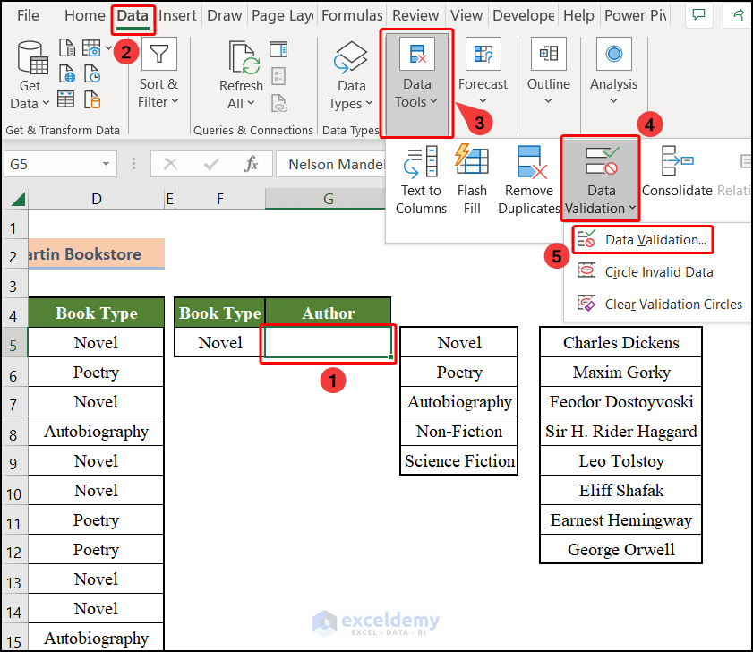
- Click on Data Validation to open the Data Validation dialog box.
- From the Allow option, select List.
- In the Source box, enter the absolute reference to the cell containing the previous formula with a HashTag (#) at the end, here $L$5#.
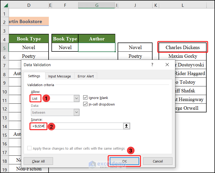
- Click on OK.
The drop-down list is generated in the selected cell.
- If you have more drop-down lists to be generated before going to the last drop-down list, follow the same procedure. For example, let’s add one more column Country after the column Author, containing the countries of the authors.

- Generate the first drop-down list (Book Type) using the process above.
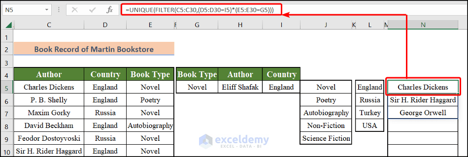
- Generate the second drop-down list (Author) based on the first drop-down list using this formula:
=UNIQUE(FILTER(C5:C30,(D5:D30=I5)*(E5:E30=G5)))
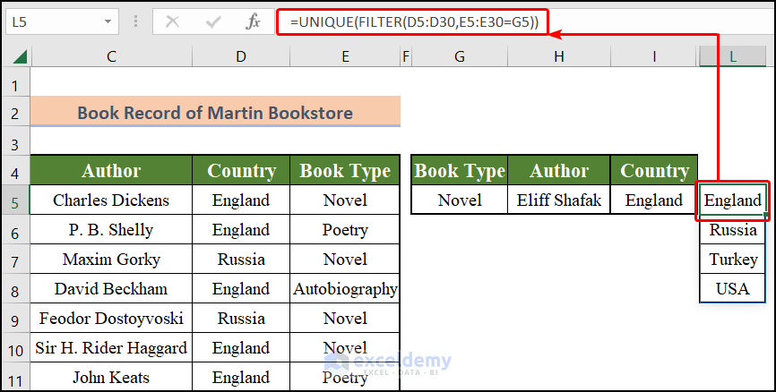
- Then generate the third drop-down list (Country) based on the first and second drop-down lists using this formula:
=UNIQUE(FILTER(D5:D30,E5:E30=G5))
- To create another drop-down list in the middle, create it based on the first, second, and third drop-down lists, and so on.
Note:
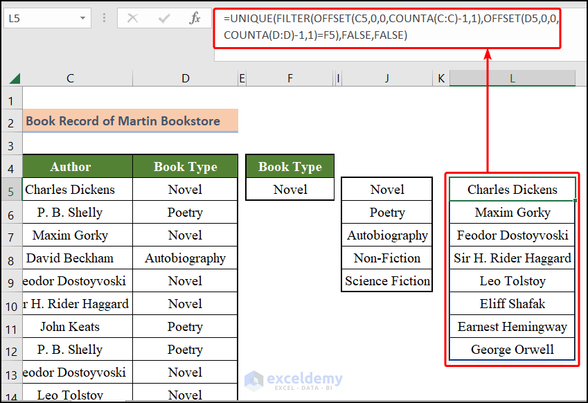
- To generate a dynamic drop-down list, use this formula instead:
=UNIQUE(FILTER(OFFSET(C5,0,0,COUNTA(C:C)-1,1),OFFSET(D5,0,0,COUNTA(D:D)-1,1)=F5),FALSE,FALSE)
As above, we replace the column arrays C5:C30 and D5:D30 with an OFFSET function of this form:
Step 3 – Create Another Dependent Drop Down List
To create the last drop-down list, we’ll use all the previous lists, but we need not use the UNIQUE function this time.
In our original data set, the last drop-down list will be of the Names of the books. This list will depend on the first and second drop-down lists.
- Select any cell in your worksheet and enter this formula:
=FILTER(B5:B30,(C5:C30=G5)*(D5:D30=F5))
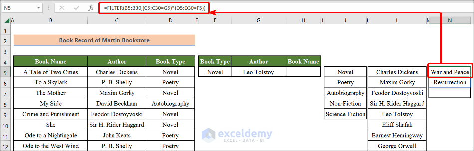
Here B5:B30 (Book Name) is the range of the last drop-down list, C5:C30 (Author) is the range of the second drop-down list, and D5:D30 (Book Type) is the range of the first drop-down list. G5 is the cell reference of the second drop-down list, and F5 is the cell reference of the first drop-down list.
- Select the cell to enter the drop-down list.
- Go to Data > Data Validation > Data Validation.
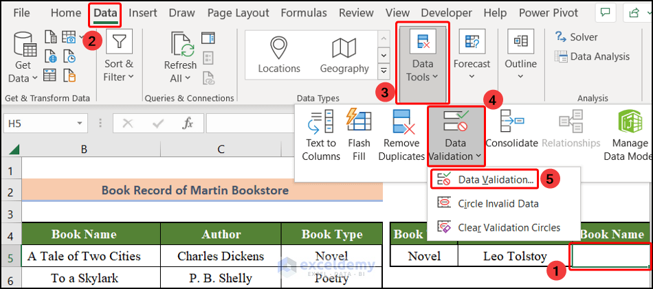
- Click on Data Validation to open the Data Validation dialog box.
- From the Allow option, select List.
- In the Source box, enter the absolute cell reference of the previous formula along with a HashTag (#) at the end, here $N$5#.
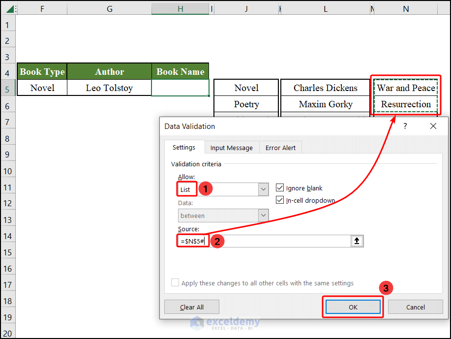
- Click OK.
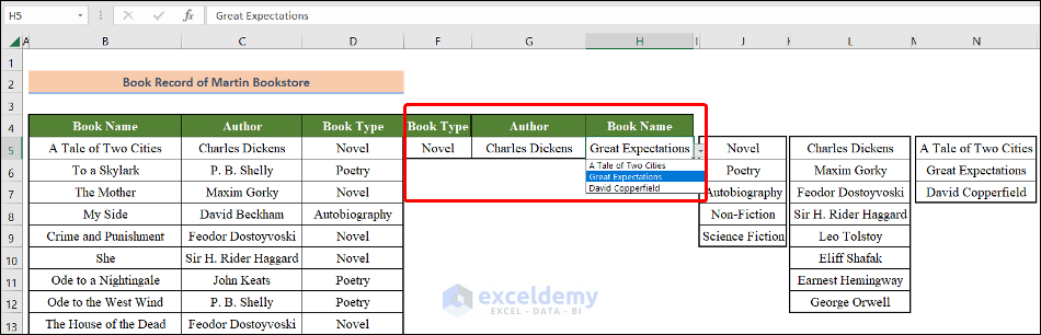
The drop-down list is generated in the selected cell.
Note:
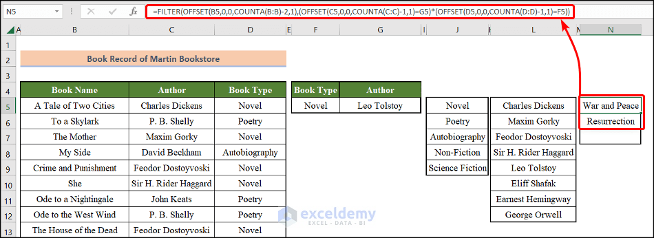
- To generate a dynamic drop-down list, use this formula instead:
=FILTER(OFFSET(B5,0,0,COUNTA(B:B)-2,1),(OFFSET(C5,0,0,COUNTA(C:C)-1,1)=G5)*(OFFSET(D5,0,0,COUNTA(D:D)-1,1)=F5))
We replace all the column arrays (C5:C30, D5:D30, and E5:E30) with an OFFSET function of this form:
Read More: How to Create Dynamic Dependent Drop Down List in Excel
Download Practice Workbook
Excel Dependent Drop Down List: Knowledge Hub
- Excel Dependent Drop Down List with Spaces
- Conditional Drop Down List in Excel
- Dynamic Dependent Drop Down List
- Dependent Drop Down List with Multiple Words in Excel
<< Go Back to Excel Drop-Down List | Data Validation in Excel | Learn Excel
Get FREE Advanced Excel Exercises with Solutions!
