How to Create a Dynamic Dependent Drop-Down List in Excel (2 Methods)

What Is Dynamic Dependent Drop-Down List?

A drop-down list is a set of predefined values from which you can choose a specific value for a cell. A dynamic dependent drop-down list consists of two parts:

1. Primary Drop-Down List (1st List): This is the initial drop-down list where you select a category or type. For example, you might choose Poetry or Science Fiction.
2. Secondary Drop-Down List (2nd List): Based on your selection from the primary drop-down list, the secondary drop-down list automatically updates to show relevant options. For instance, if you choose Poetry, the second list will display book names related to poetry.

Method 1 – Using Formulas to Create a Dynamic Dependent Drop-Down List

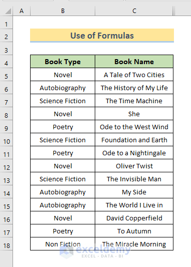
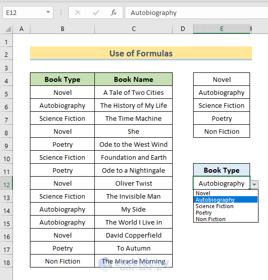
We’ll assume you have a dataset containing two columns: Book Type and Book Name.

Step 1 – Creating the Primary Drop-Down List

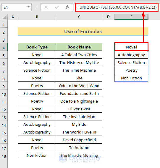
• In Cell E4, enter the following formula to create the list of unique book types:

• Press Enter, and an array of book types will be generated.

• Select the cell where you want to create the primary drop-down list (e.g., Cell E12).
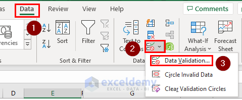
• Go to the Data tab and choose Data Validation.

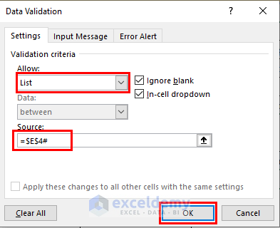
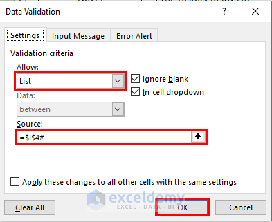
• In the Data Validation window:
  • Select List in the Allow section.
  • In the Source box, enter $E$4#.
• Press OK. You’ll now see a drop-down list in Cell E12, allowing you to select different book types.

• We will see a drop-down list in Cell E12. We can select different Book Types from there.

Step 2 – Inserting the Second Drop-Down List

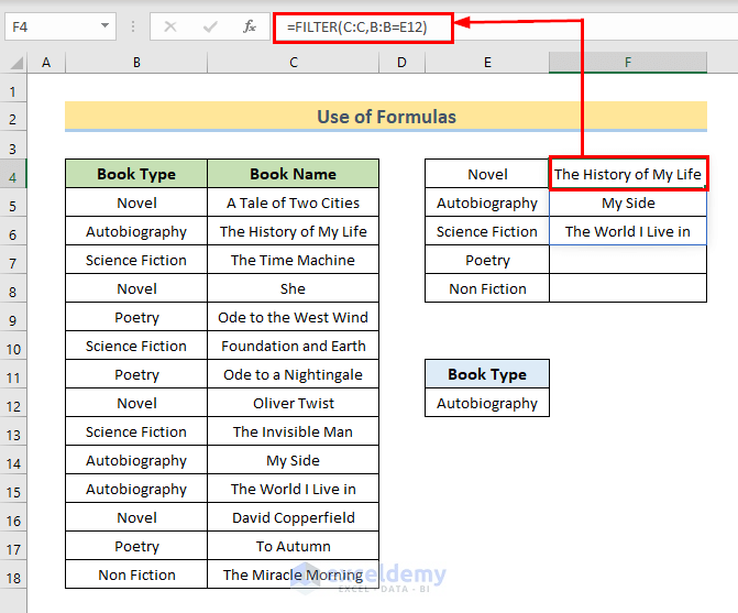
• In Cell F4, enter the following formula to create the list of Book Names based on the selected book type:

• Press Enter, and the Book Names related to the chosen book type will appear.

• Select Cell F12 and go to the Data tab.
• Choose Data Validation.

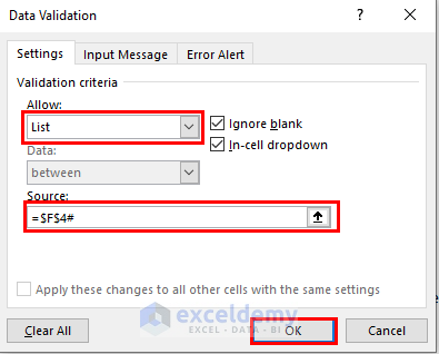
• In the Data Validation window:
  • Select List in the Allow section.
  • In the Source box, enter $F$4#.
• Press OK.

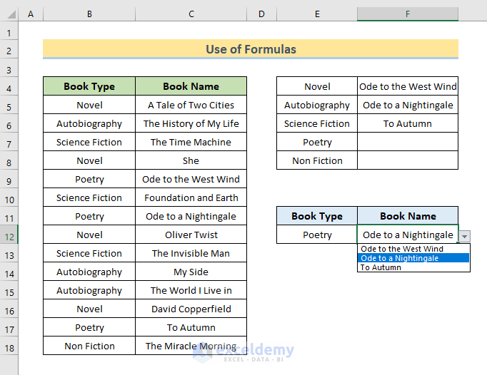
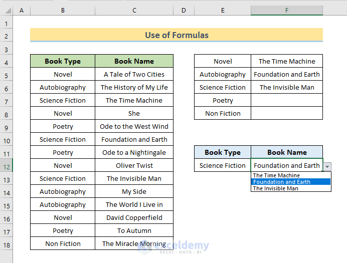
• Now you have a dynamic dependent drop-down list.

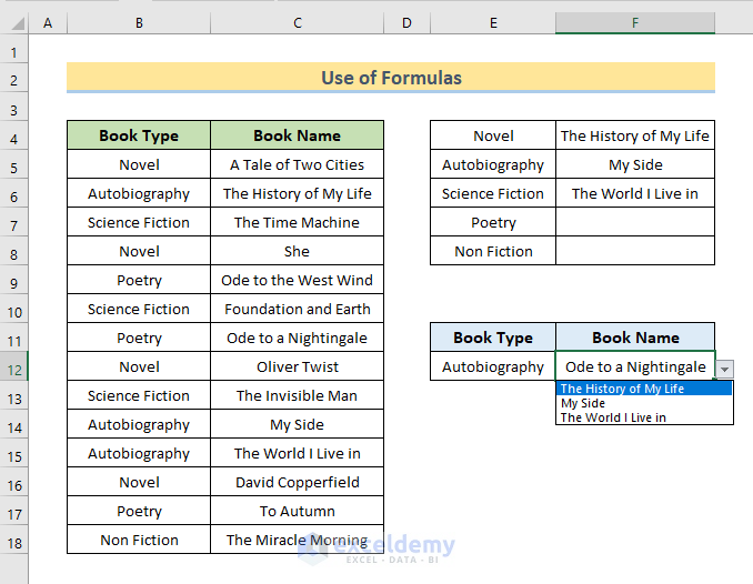
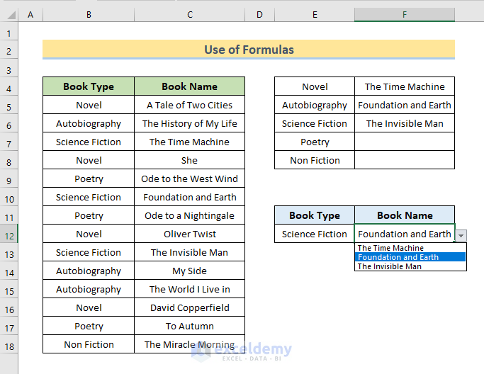
• If you change the selection in the first drop-down list, the content of the second drop-down list will automatically update to match the chosen book type.

Read More: How to Create Dependent Drop-Down List with Multiple Words in Excel

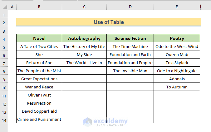
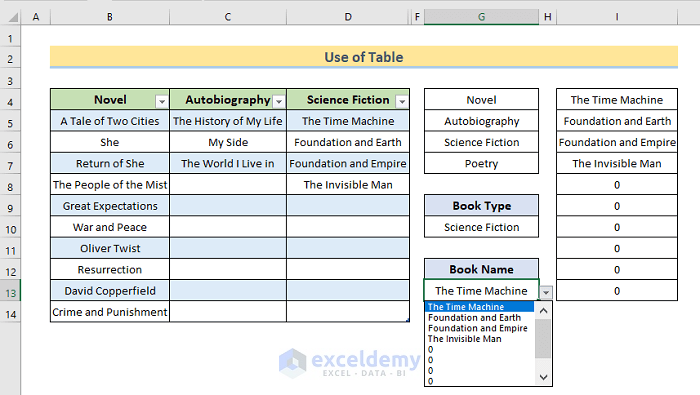
Method 2 – Using Excel Table to Create Dynamic Dependent Drop-Down List

In this method, we’ll create a dynamic dependent drop-down list using an Excel table. For demonstration purposes, I’ve used different book names categorized under columns such as Novel, Autobiography, Science Fiction, and Poetry.

Step 1 – Creating the Primary Drop-Down List

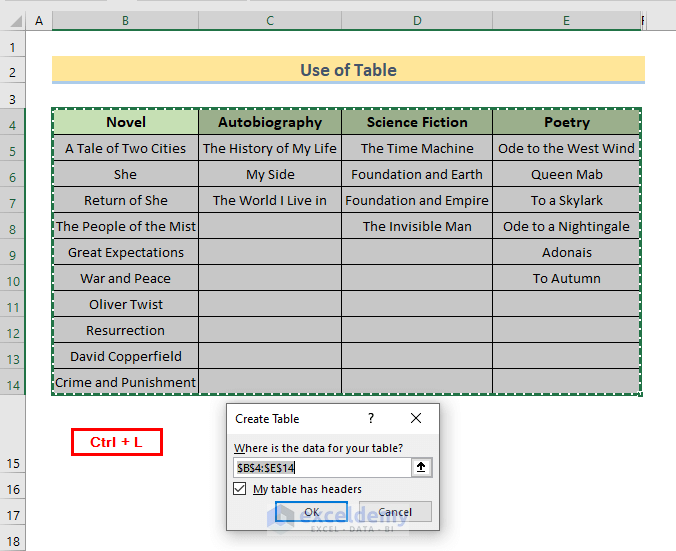
• Create the Table:
  • Select the entire dataset (including the book names and categories).
  • Press Ctrl + L to create an Excel table.
  • In the Create Table window, press OK.

• Generate the Primary List:
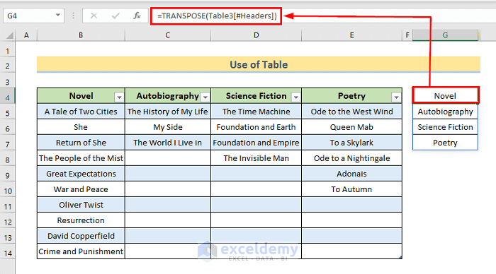
  • Enter the following formula in Cell G4:

(Replace Table3 with the actual name of your table if it’s different.)

• • The primary list (book categories) will be created in Cell G4.

• Data Validation for Primary List:
  • Select Cell G10.
  • Go to the Data tab.
  • Choose Data Validation.

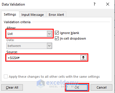
• In the Data Validation window:
  • Select List in the Allow section.
  • In the Source section, enter $G$4#.
• Press OK.

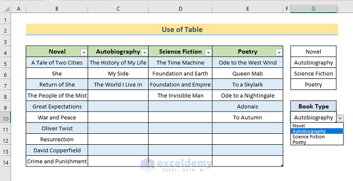
• Now you can select different book types from the primary drop-down list.

Step 2 – Generating the Second Drop-Down List

• Create the Dynamic-Dependent List:
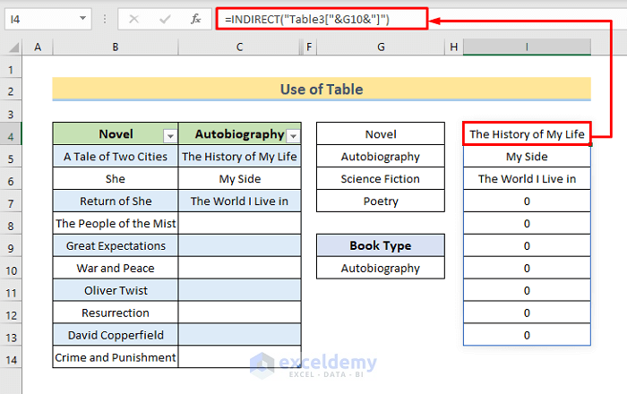
  • Enter the following formula in Cell I4:

• • Press Enter, and the second list (book names related to the selected category) will appear in Cell I4.

• Data Validation for Second List:
  • Select Cell G13.
  • Go to the Data tab.
  • Choose Data Validation.

• • In the Data Validation window:
    • Select List in the Allow section.
    • In the Source section, select Cell $I$4 with a # sign at the end.
  • Press OK.

• You will see the drop-down list in Cell G13.

• Now you have a dynamic dependent drop-down list. If you change the selection in the first drop-down list, the content of the second drop-down list will automatically update to match the chosen book category.

Read More: Create Excel Drop Down List from Table

Download Practice Workbook

You can download the practice workbook from here:

Related Articles

• Conditional Drop Down List in Excel
• How to Use IF Statement to Create Drop-Down List in Excel
• Excel Dependent Drop Down List
• How to Make Dependent Drop Down List with Spaces in Excel
• Create Excel Filter Using Drop-Down List Based on Cell Value
• Excel Formula Based on Drop-Down List
• How to Extract Data Based on a Drop Down List Selection in Excel
• How to Populate List Based on Cell Value in Excel
• How to Change Drop Down List Based on Cell Value in Excel

<< Go Back to Excel Dependent Drop Down List | Excel Drop-Down List | Data Validation in Excel | Learn Excel