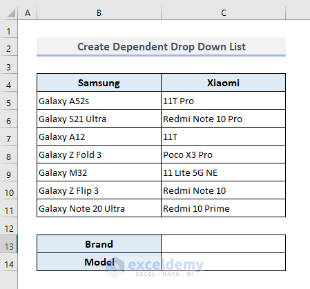
Method 1 – Create a Conditional Drop-Down List with a Classified Data Table
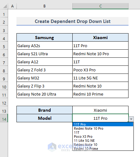
In Cell C13, we’ll create an independent drop-down list for the brand types. After that, we’ll make a dependent drop-down list in Cell C14 where smartphone models will be shown in a list based on the selected brand from the previous drop-down list.
Steps:
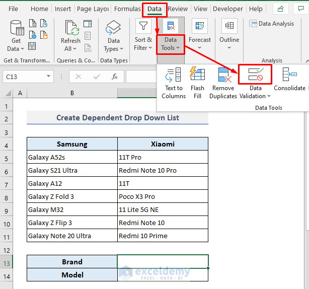
- Select cell C13.
- Under the Data tab, choose the Data Validation command from the Data Tools drop-down.
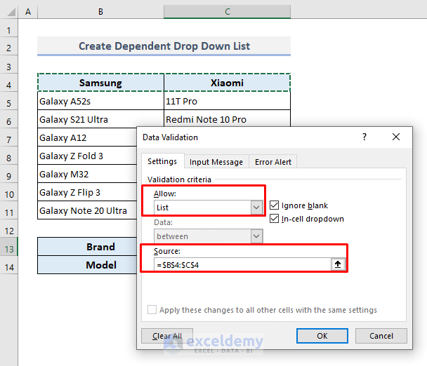
- In the Allow box, select List from the options.
- Click in the Source box and select the range of cells (B4:C4) containing the brand names of the smartphones.
- Press OK.
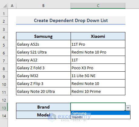
- This creates an independent drop-down list for the smartphone brands in cell C13.
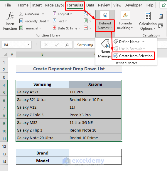
- Select the entire table or the range of cells B4:C11.
- Under the Formulas ribbon, choose the Custom from Selection command from the Defined Names drop-down.
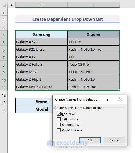
- A dialogue box will appear.
- Check Top row only and leave other options unmarked.
- Press OK.
- This creates two named ranges for two different smartphone brands with their corresponding models.
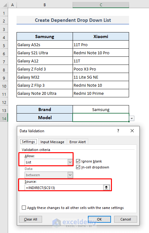
- Since we have to create a dependent drop-down list in Cell C14, select it.
- Go to Data Validation again.
- Choose List in the Allow box.
- In the Source box, copy the following formula:
=INDIRECT($C$13)- Press OK.
By using the INDIRECT function here, we’ve mentioned the cell reference of C13. The function will store the smartphone models in arrays for two different brands.
- Select a smartphone brand from the independent drop-down in cell C13 and then click on the dependent drop-down button in cell C14. You’ll find all the smartphone models of the selected brand.
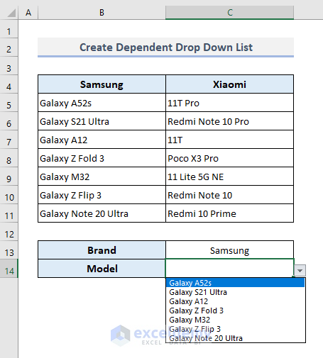
- Alter the smartphone brand and you’ll find the corresponding smartphone models only, as shown in the screenshot below.
Read More: How to Use IF Statement to Create Drop-Down List in Excel
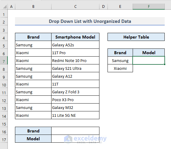
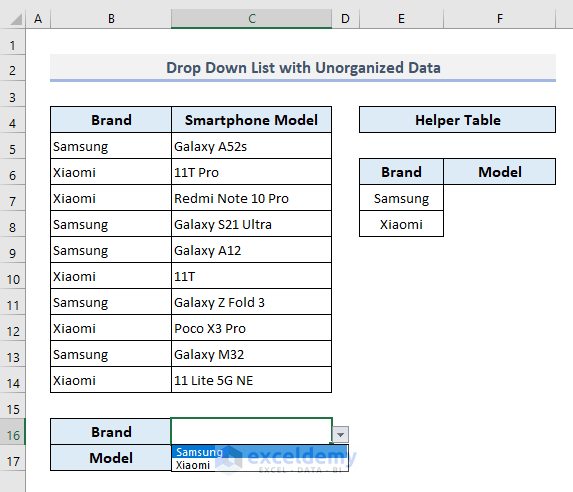
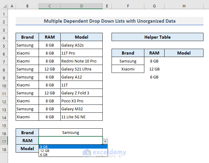
Method 2 – Make a Conditional Drop-Down List with an Unorganized Data Table
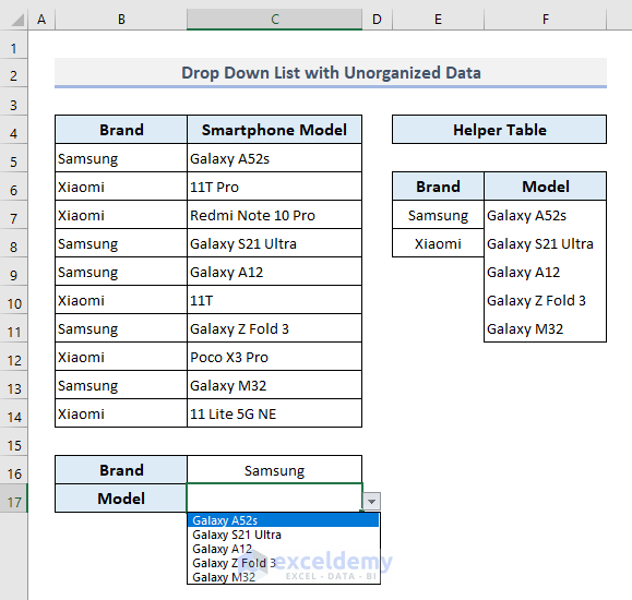
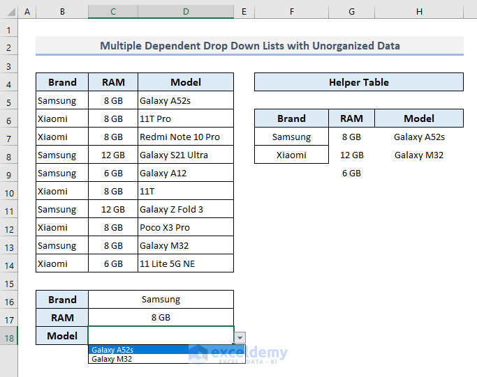
In this data table, we’ll make a dependent drop-down list in cell C17. We’ll use a helper table where we’ll store the filtered smartphone models based on the selection from the independent drop-down.
Steps:
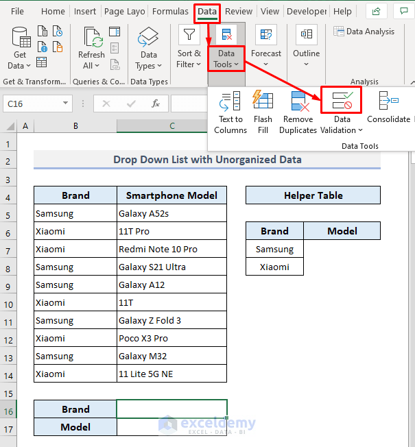
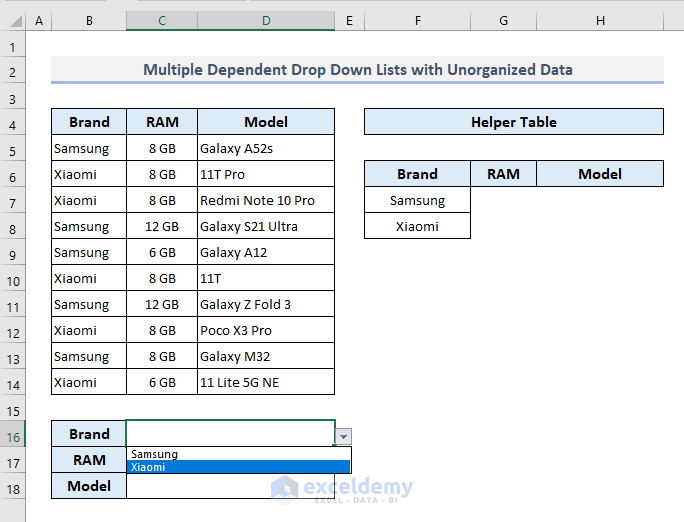
- Select Cell C16 to make an independent drop-down list first for the brand names.
- Under the Data tab, choose the Data Validation option from the Data Tools drop-down.
- A dialogue box will open up.
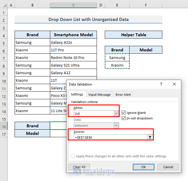
- In the Allow box, select List from the options.
- In the Source box, put the range of cells (E7:E8) containing the brand names.
- Press OK.
- Select an option in the new drop-down. We put Samsung.
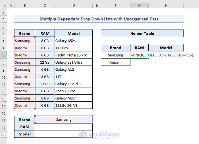
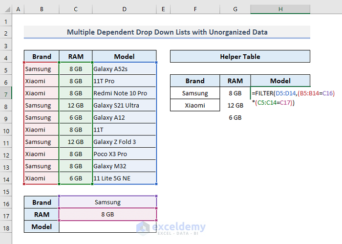
- Select Cell F7 and copy the following formula into it:
=FILTER(C5:C14,B5:B14=C16)- Press Enter.
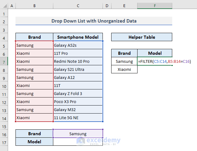
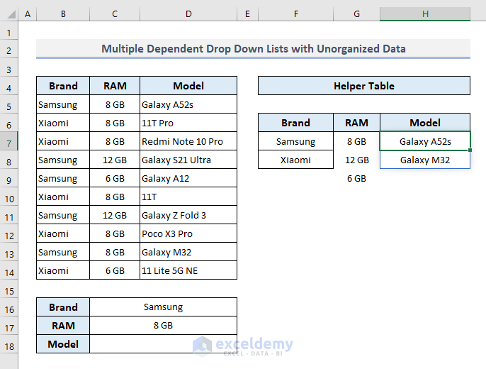
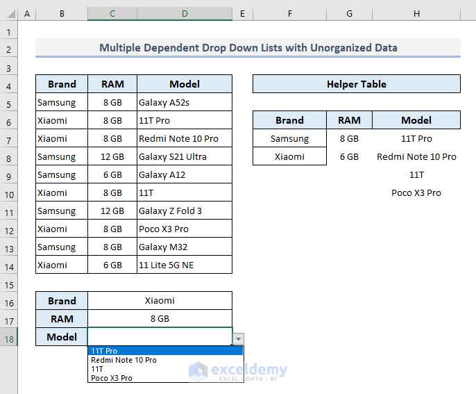
- You’ll find all models of the Samsung brand here in a vertical array under the Model header in the Helper Table.
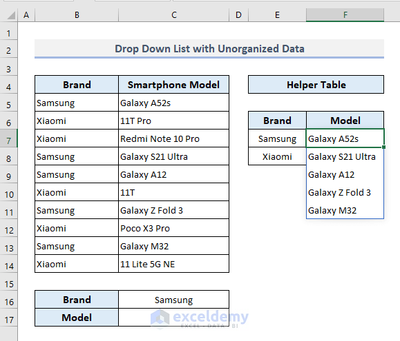
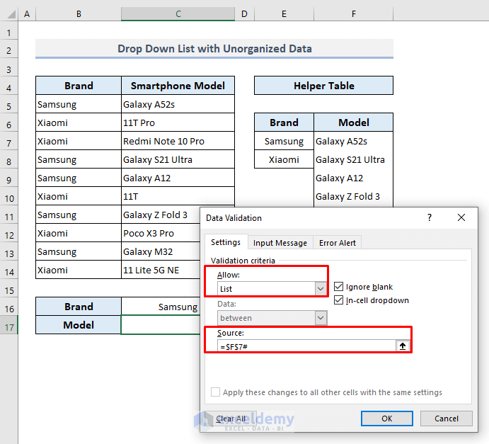
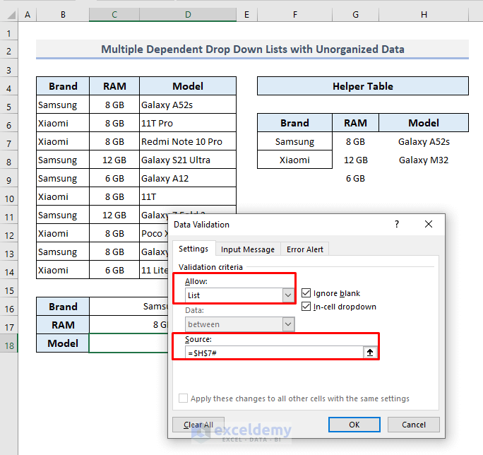
- Select cell C17.
- Go to the Data Validation option again.
- Select List in the Allow box.
- In the Source box, input:
=$F$7#With the use of Hash (#) here, we’re defining the spill range starting from Cell C17.
- Press OK.
- The dependent drop-down list shows the assigned items.
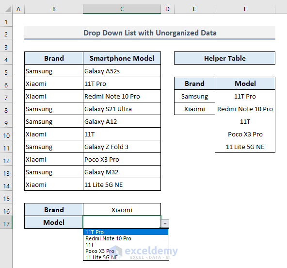
- Alter the brand name from the Brand drop-down and you’ll find the corresponding smartphone models in the Model drop-down list.
Read More: Excel Formula Based on Drop-Down List
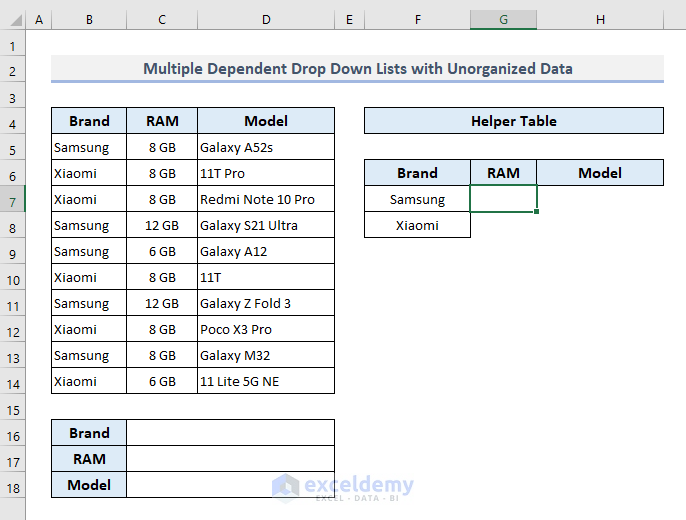
Method 3 – Construct Multiple Conditional Drop-Down Lists in Excel
In our data table, we’ve added a new column with the RAM header. We’ll create two conditional drop-down lists here in Cells D17 and D18, one is for RAM and another one is for the smartphone model. Once we select the available RAM first from the drop-down list based on the selected smartphone brand, the corresponding smartphone models will show up in the second dependent drop-down.
Steps:
- Select Cell C16 and open Data Validation.
- Choose the option List in the Allow box.
- Select the range of cells (F7:F8) containing the brand names for the Source box.
- Press OK.
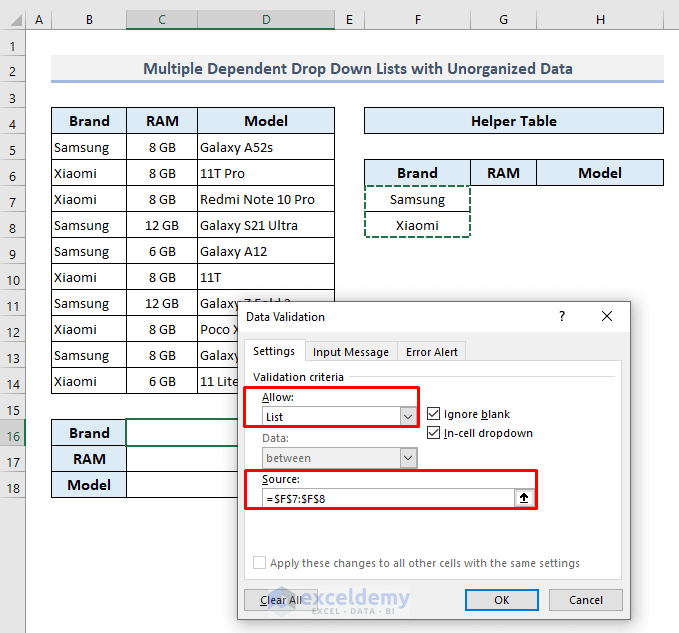
- This creates an independent drop-down in Cell C16 for brand names.
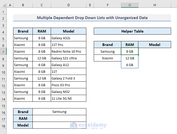
=UNIQUE(FILTER(C5:C14,B5:B14=C16))- Press Enter.
We’re using the UNIQUE function here to show each different RAM only once in the spill range.
- You’ll get a vertical array in Cell G7 with the available RAMs from the data table for the devices chosen in the drop-down.
- Select Cell C17.
- Open Data Validation.
- Select List from the options in the Allow box.
- In the Source box, put:
=$G$7#- Press OK.
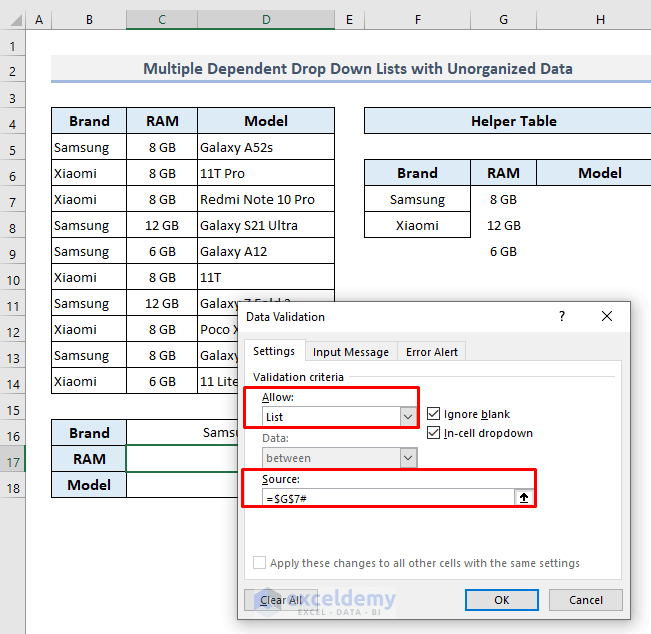
- The first dependent drop-down list is now complete. Once you click on the drop-down from Cell C17, you’ll find the available RAMs for the selected smartphone brand.
- Select Cell H7 and insert the following:
=FILTER(D5:D14,(B5:B14=C16)*(C5:C14=C17))- Press Enter.
In this cell, we’re now assigning the model names for the selected brand and RAM with the FILTER function.
- The smartphone model names that follow the selected criteria are visible with a spilled range from Cell H7.
- Select Cell C18 to create the second drop-down list.
- Open Data Validation.
- Choose List in the Allow box from the options.
- In the Source box, copy the following:
=$H$7#- Press OK.
- You’ll see the filtered smartphone model names in the drop-down list in Cell C18.
- Alter the brand name and RAM from the first two dropdowns, and you’ll be displayed the corresponding device models in the drop-down list in Cell C18
Read More: How to Create Dependent Drop Down List with Multiple Words in Excel
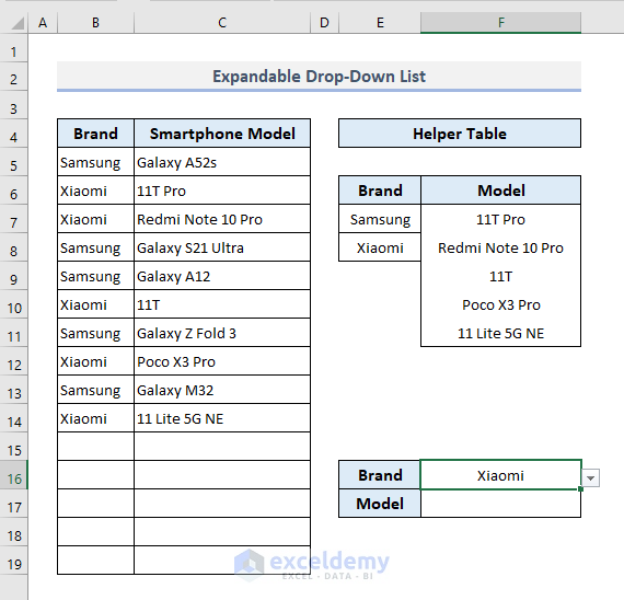
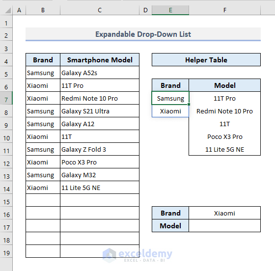
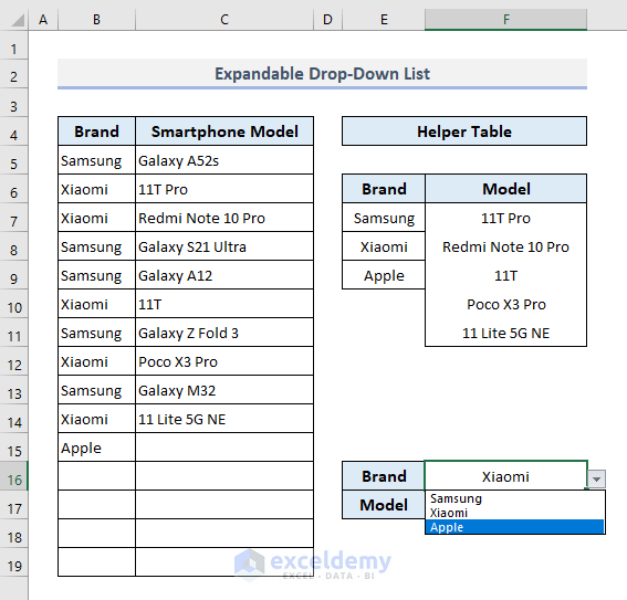
Method 4 – Prepare an Expandable Drop-Down List in Excel
Let’s add five more rows to the dataset from Method 2 and move the dropdowns out of the way. The new rows aren’t included in the original formulas, so the filters and dropdowns can’t fetch data from it. Let’s make some modifications to allow the drop-down lists to work with the newly added data in the table.
Steps:
- Select Cell E7 and copy the following formula into it:
=UNIQUE(FILTER(B5:B19,B5:B19<>""))- Press Enter.
This formula filters the values from the range of cells (B5:B19) in Column B to show each different brand name only once. It will ignore the empty cells.
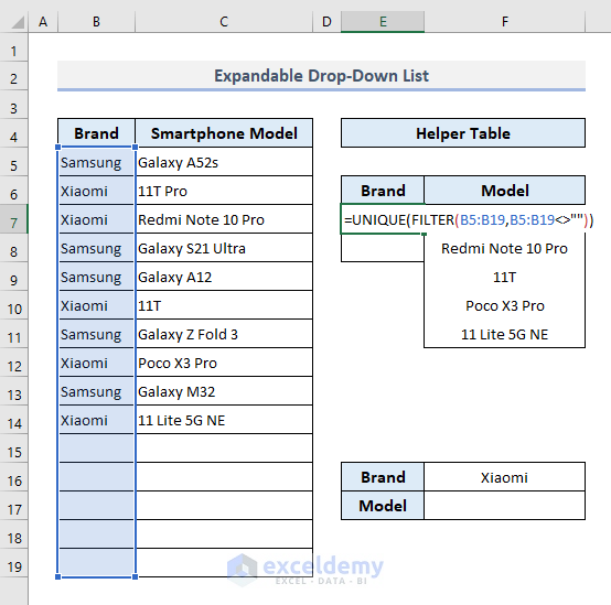
- Starting with Cell E7, the brand names are now visible in a spill range.
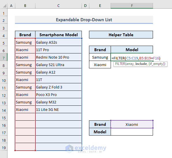
- Select Cell F7 and insert the following:
=FILTER(C5:C19,B5:B19=F16)- Press Enter.
This formula defines the smartphone models based on the selected brand from the drop-down list in Cell F16.
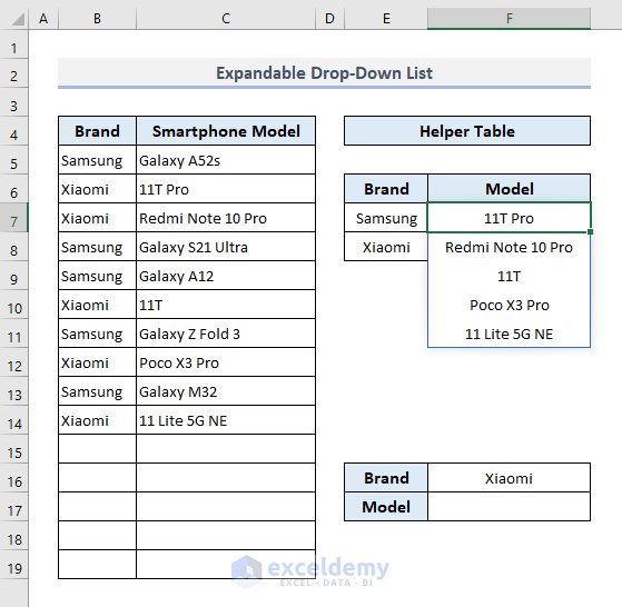
- The available smartphone models from the brand chosen in cell F16 will be shown in a vertical array from Cell F7.
- Select Cell F16 now and go to Data Validation.
- Choose List from the options in the Allow box.
- In the Source box, input:
=$E$7#- Press Enter.
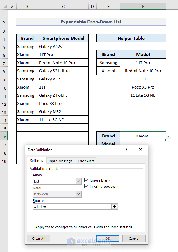
- The drop-down now uses the spill range of unique values from the E column. If you click on the Brand drop-down, you’ll find the updated brand names in the list.
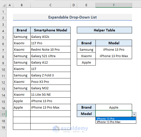
- Add some smartphone models in the table for the corresponding brand and you’ll find those newly added names of the devices in the Model drop-down list. This is how you can easily create an expandable drop-down list with the referred steps.
Sort a Conditional Drop-Down List in a Specified Order
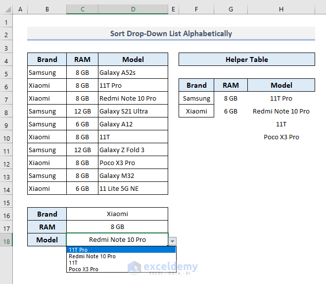
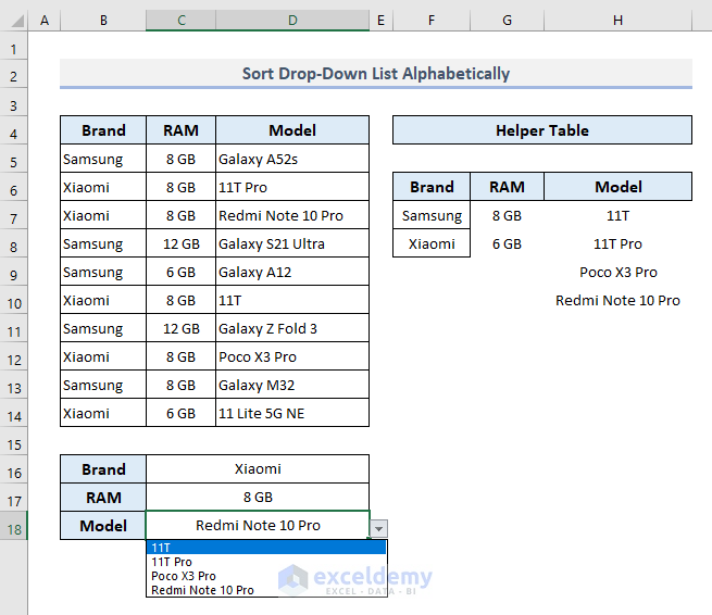
Method 1 – Sort a Dependent Drop-Down List in Alphabetical Order in Excel
Let’s use the dataset from Method 3 in the previous section. The drop-down values are sorted based on the order they appear in the dataset and filtered in column F. Let’s sort them alphabetically (From A to Z) by modifying the formula in Cell H7.
- In Cell H7, the modified formula combining the SORT and FILTER functions will be:
=SORT(FILTER(D5:D14,(B5:B14=C16)*(C5:C14=C17)),,1)In this formula, we’re defining the order with ‘1’ in the third argument (sort_order) of the SORT function. This will sort the data in ascending order (from A to Z for alphabets). If we use ‘-1’ as the sort_order, it’ll denote the descending order for numerical data and Z to A for alphabets.
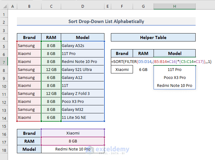
- Press Enter, and the formula will return the sorted data from Cell H7 as shown in the picture below.
- Click on the Model drop-down icon and you’ll find the items in the specified order. Items starting with numerical characters will always be at the beginning.
Method 2 – Sort a Conditional Drop-Down List with an Ascending or Descending Order
Let’s sort the memory storage of the RAMs now that are visible from Cell G7 with a spilled range. The RAM drop-down list also stores the order followed by that spilled range.
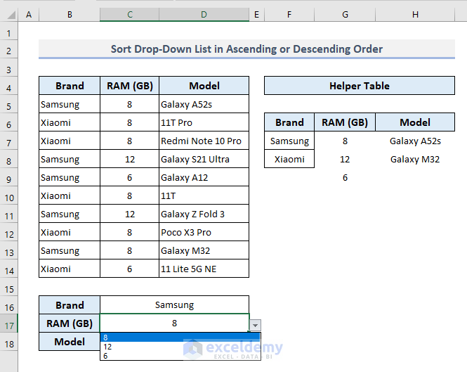
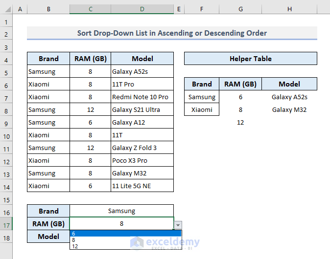
- Insert the following formula in Cell G7 and press Enter.
=SORT(UNIQUE(FILTER(C5:C14,B5:B14=C16)),,1)
- The spilled range from Cell G7 will show the numerical values in ascending order. Now click on the RAM drop-down and you’ll find the items too in the specified order.
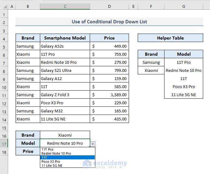
How to Use a Conditional Drop-Down List in Excel: A Practical Example
In the following dataset, the Price column has been added to the primary table containing two smartphone brands and corresponding model names only. We’ll select a brand and the corresponding smartphone model and then display the price of the product with a lookup function.
For example, we want to display the price of the handset ‘Xiaomi 11T’ after two selection processes from the drop-down lists.
Steps:
- Select Xiaomi from the Brand drop-down list first.
- Choose the handset model 11T from the Model drop-down list.
- In the output Cell C18, where the price will be displayed, insert the following formula:
=XLOOKUP(C17, C5:C14, D5:D14)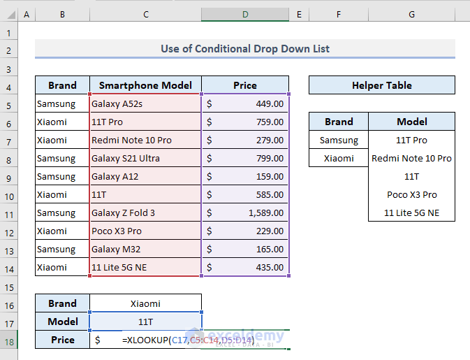
- Press Enter and you’ll get the result based on the criteria chosen in the drop-down lists.
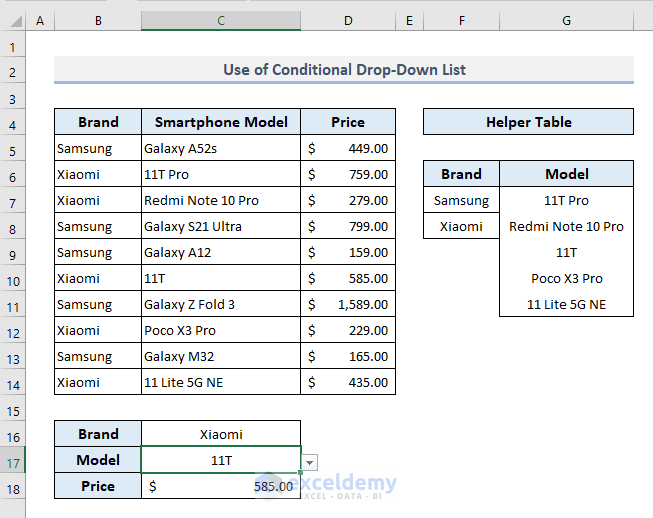
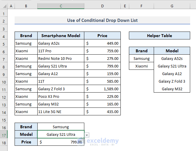
- Change the smartphone brand and the corresponding model from the drop-down lists.
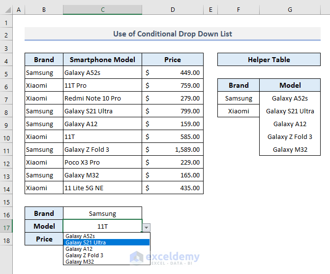
- The output data in Cell C18 will be updated immediately for the newly selected device.
Download Practice Workbook
You can download the Excel workbook that we’ve used to prepare this article.
Related Articles
- How to Create Dynamic Dependent Drop Down List in Excel
- How to Make Dependent Drop Down List with Spaces in Excel
- Create Excel Filter Using Drop-Down List Based on Cell Value
- How to Extract Data Based on a Drop Down List Selection in Excel
- How to Populate List Based on Cell Value in Excel
- How to Change Drop Down List Based on Cell Value in Excel
<< Go Back to Excel Dependent Drop Down List | Excel Drop-Down List | Data Validation in Excel | Learn Excel
Get FREE Advanced Excel Exercises with Solutions!

This is great and has solved my problems using dependent dropdown lists but can conditional drop down lists work for multiple rows?
Hello Kris! I am assuming that you are trying to do something as follows.
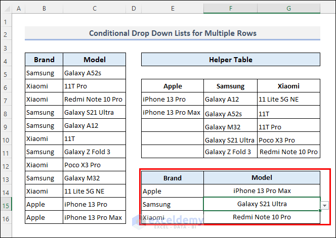
You can apply the following steps to be able to do that.
First, enter the following formula in cell E6.
=TRANSPOSE(SORT(UNIQUE(B5:B16)))Then, apply the following formula in cell E7.
=SORT(FILTER($C$5:$C$16,$B$5:$B$16=E$6))Next, drag the fill handle icon to the right.
After that, enter =$E$6# as the source for data validation in cell E14.
Then, drag the fill handle icon below.
Next, enter the following formula as the source for data validation in cell F14.
=INDIRECT(ADDRESS(7, COLUMN(D1) + MATCH(E14, $E$6#, 0), 4) & "#")Now copy the cell. Then select multiple cells below it. Next, paste it there as validation using paste special.
Thanks, that was very useful. However I need to create a conditional drop down from a classified data list but where the list is on another Excel worksheet (in the same workbook). Is that possible? I can’t get it to work following the method above.
Hello JUILA! I hope you are fine. You can easily create a conditional drop-down list from other worksheets in the same workbook. You can follow this article-
https://www.exceldemy.com/excel-drop-down-list-from-another-sheet
This article will show you the process step-by-step with proper illustrations. Try the methods mentioned in this article and let us know the outcome. Thank you!