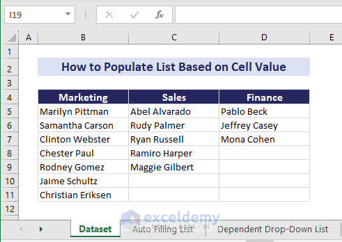
We have the employee names of the respective departments. We’ll populate the list of employees based on a department.
Method 1 – Populating a Data Validation Drop-Down List Based on Cell Value in Excel
The sample dataset contains employees of 3 different departments. We’ll populate a drop-down list with employee names based on the department we select. Then, we can select employee names from the drop-down options to fill the list when needed.
Part 1.1 – Creating a Dependent Drop-Down List Using the INDIRECT Function
Steps:
- Select the range B7:D13.
- Type Marketing in the Name Box to name the cell range. Note that the named range doesn’t include the header.
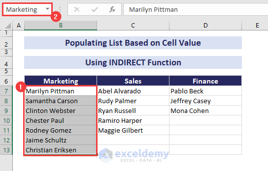
- Name the respective cell ranges for the Sales and Finance departments.
- Select the range B16:B22 and go to the Data tab.
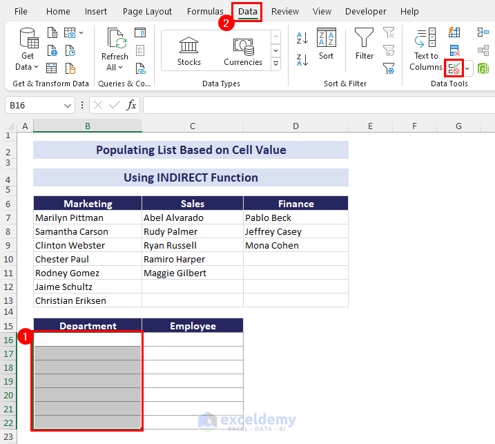
- Select Data Validation from the Data Tools group.
- Choose List in the Allow field.
- Set B6:D6 as the Source.
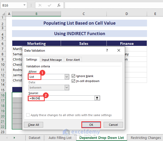
- Press OK to close the dialog box.
- We created the drop-down list of departments. Click the drop-down icon and you’ll see the available options.

- Select the range C16:C22.
- Go to the Data tab.
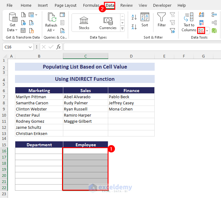
- In the Data Tools group, select Data Validation.
- Choose List in the Allow field.
- Insert the following formula in the Source field:
=INDIRECT(B16)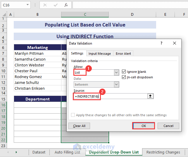
- Press OK to close the dialog box.
- Select Sales from the department drop-down. The corresponding drop-down list in C16 will display the employee names from the Sales department only.
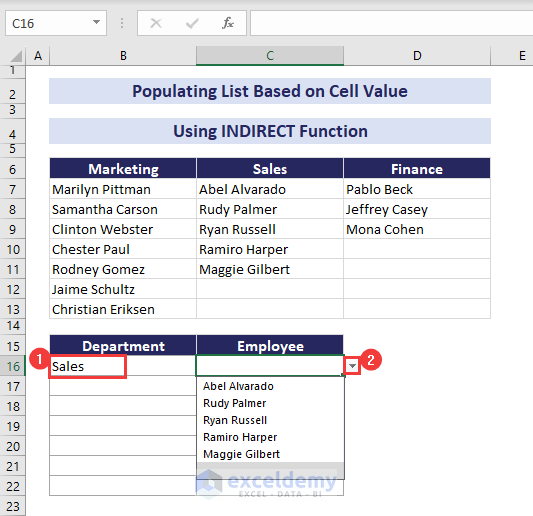
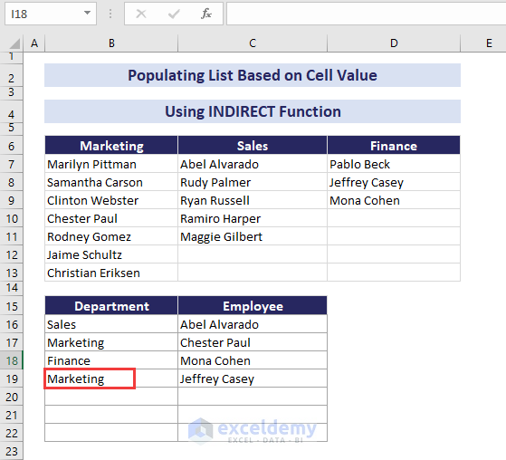
- You can populate the list by selecting from the drop-down options. We’ve filled a portion of the list in the following picture.

- Change the department in cell B19 from Finance to Marketing. However, the corresponding employee name in cell C19 still stays, which needs to be fixed.
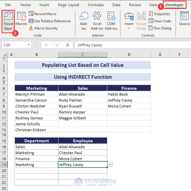
- Go to the Developer tab and select Visual Basic.
- In the VBA window, double-click on Sheet2 (Dependent Drop-Down List) from the Microsoft Excel Objects.
- In the code window, paste the following code:
Private Sub Worksheet_Change(ByVal Target As Range)
On Error Resume Next
If Target.Column = 2 Then
 If Target.Validation.Type = 3 Then
 Application.EnableEvents = False
 Target.Offset(0, 1).ClearContents
 End If
End If
exitHandler:
 Application.EnableEvents = True
 Exit Sub
End Sub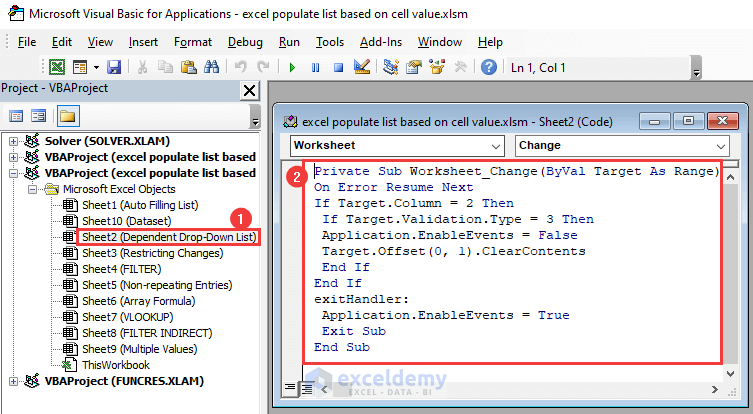
- Save the file and close the VBA window.
- Change a department in the drop-down list on the left. The corresponding employee’s name will be cleared immediately.
Read More: How to Create Dynamic Dependent Drop Down List in Excel
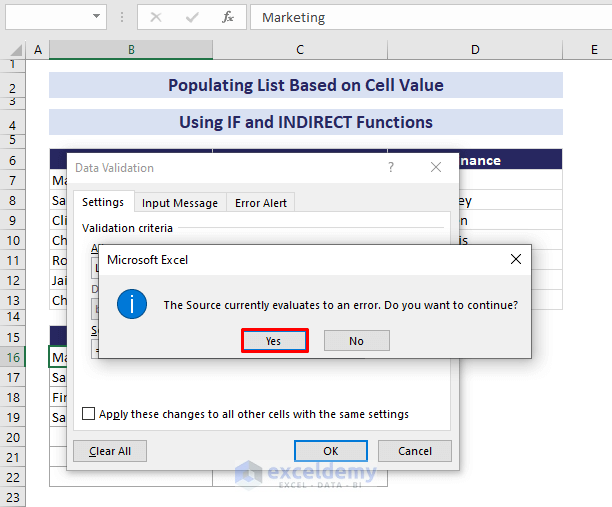
Part 1.2 – Restricting Changes in the First Drop-Down List Using IF and INDIRECT Functions
- Open the Data Validation after selecting the cell range for departments.
- Choose List in the Allow field and insert the following formula in the Source field:
=IF(B16="",Department, INDIRECT("FakeRange"))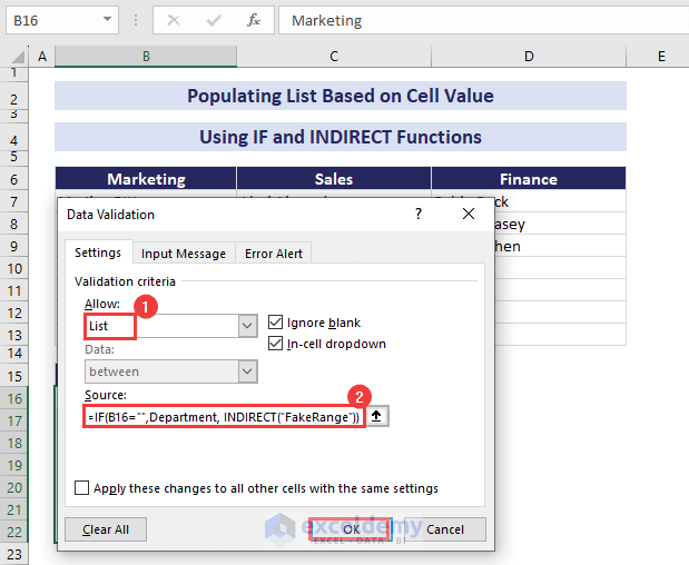
- Press OK to close the dialog box.
- A warning message box will pop out. Click Yes.
- Click the drop-down of the already inserted department. It’ll have no effect.
![]()
Read More: How to Use IF Statement to Create Drop-Down List in Excel
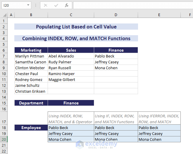
Method 2 – Combining INDEX, ROW, and MATCH Functions to Automatically Populate a List Based on Cell Value
Steps:
- Select cell C15.
- Go to the Data tab.

- Select Data Validation from the Data Tools group. The Data Validation dialog box appears.
- In the Allow field, choose List from the drop-down.
- Select B6:D6 as the Source.
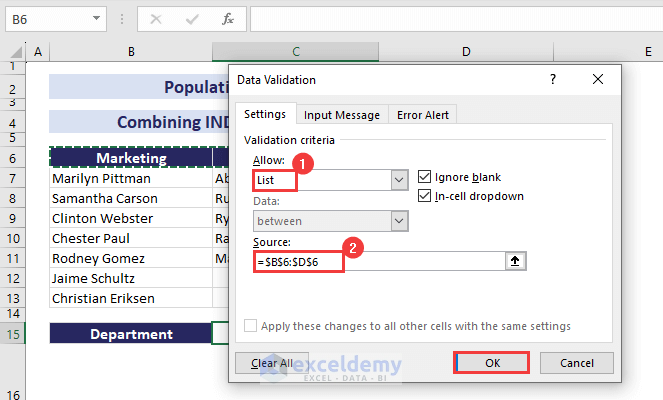
- Press OK.
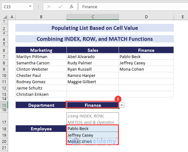
- The department drop-down list appears in cell C15. You can choose any of them.
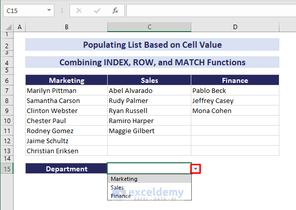
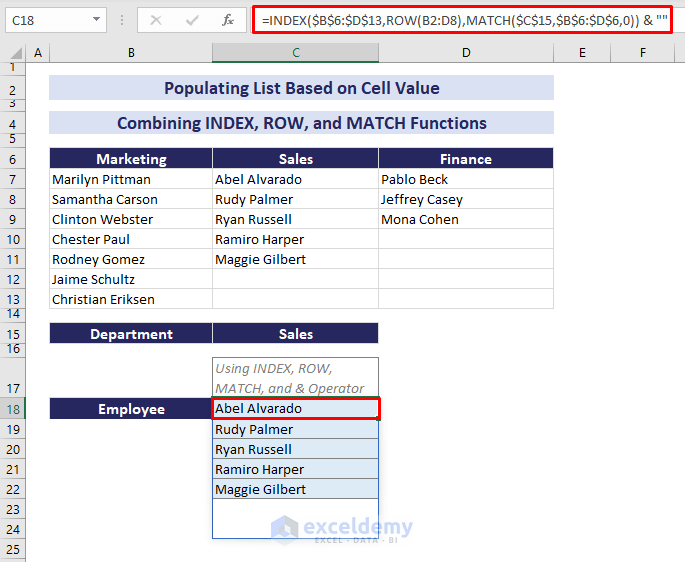
- Select cell C18 and insert the following formula:
=INDEX($B$6:$D$13,ROW(B2:D8),MATCH($C$15,$B$6:$D$6,0)) & ""- Press Enter.
- It’ll spill the employee list of the department from cell C15.
- Change the department to Finance. The list will get updated automatically.
Formula Breakdown
=INDEX($B$6:$D$13,ROW(B2:D8),MATCH($C$15,$B$6:$D$6,0)) & “”
=INDEX($B$6:$D$13,ROW(B2:D8),3) & “” // MATCH($C$15,$B$6:$D$6,0) returns 3 because C15 (Finance) is matched in position 3 in the range B6:D6.
=INDEX($B$6:$D$13,{2;3;4;5;6;7;8},3) & “” // ROW(B2:D8) returns {2;3;4;5;6;7;8} because the ROW function returns the row number of the cell references.
=Pablo Beck & “” // INDEX($B$6:$D$13,{2;3;4;5;6;7;8},3) returns Pablo Beck because the intersection of row 2 and column 3 in the range B6:D12 is Pablo Beck.
=Pablo Beck // Because concatenating with “” using the & operator still returns Pablo Beck.
As our formula is a dynamic array formula, it spills all the values present in the intersection of each of the rows 2 to 8 and column 3.
If no value is found, it returns 0, but concatenating 0 with “” using the & operator results in an empty string, thus we see blank cells.
- We can also use the below formula with the IF function to return blank cells instead of 0 when auto-populating a list based on cell value.
=IF(INDEX($B$6:$D$13,ROW(B2:D8),MATCH($C$15,$B$6:$D$6,0))<>0, INDEX($B$6:$D$13,ROW(B2:D8),MATCH($C$15,$B$6:$D$6,0)), "")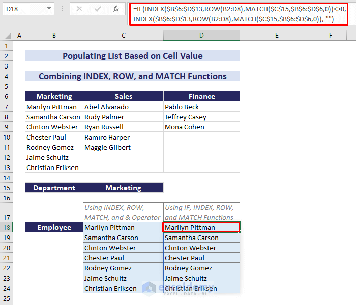
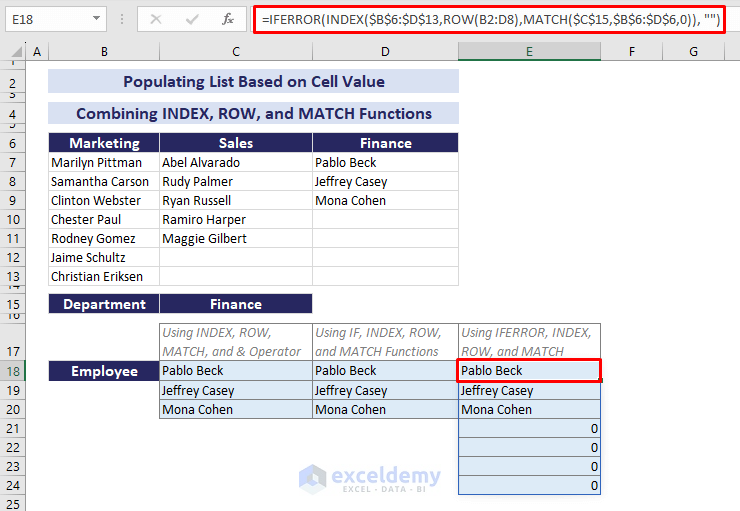
- We can apply Conditional Formatting to make the 0 values invisible by making the font color white wherever we find them. The formula used is:
=IFERROR(INDEX($B$6:$D$13,ROW(B2:D8),MATCH($C$15,$B$6:$D$6,0)), "")It’s pretty much the same formula as we used earlier, the additional IFERROR function here will return blanks if any error is encountered.
To apply Conditional Formatting:
- Select the desired range.
- Select Conditional Formatting drop-down.
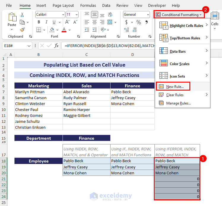
- Click New Rule. The New Formatting Rule dialog appears.
- Choose Format only cells that contain rule type.
- In the Format only cells with fields, select Cell Value, equal to, and 0 for the three boxes, respectively.
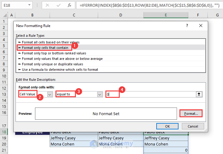
- Click Format.
- In the Format Cells dialog box, go to Font and choose White as Color.
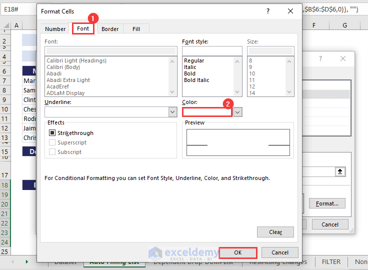
- Press OK to close the Format Cells dialog box.
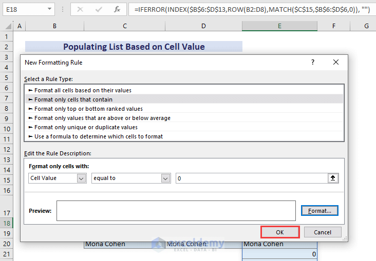
- Press OK to close the New Formatting Rule dialog box.
The following GIF displays the dynamic list generation whenever we change the department.
Read More: Excel Formula Based on Drop-Down List
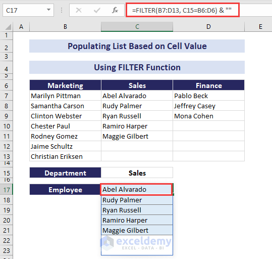
Method 3 – Inserting the FILTER Function for Populating a List Based on Cell Value in Excel
Steps:
- The department selection in C15 is created via Data Validation drop-down as shown in the previous methods.
- Select cell C17.
- Insert the following formula:
=FILTER(B7:D13, C15=B6:D6) & ""- Press Enter. The respective employee list will get spilled depending on the department in cell C15.
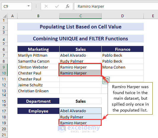
Method 4 – Combining UNIQUE and FILTER Functions to Populate the List with Non-repeating Entries
Steps:
- Put a Data Validation drop-down in C15 for the department (see Method 1).
- Select cell C17.
- Insert the following formula:
=UNIQUE(FILTER(B7:D13, C15=B6:D6)) & ""- Press Enter and the formula will spill the employee list of the respective department.
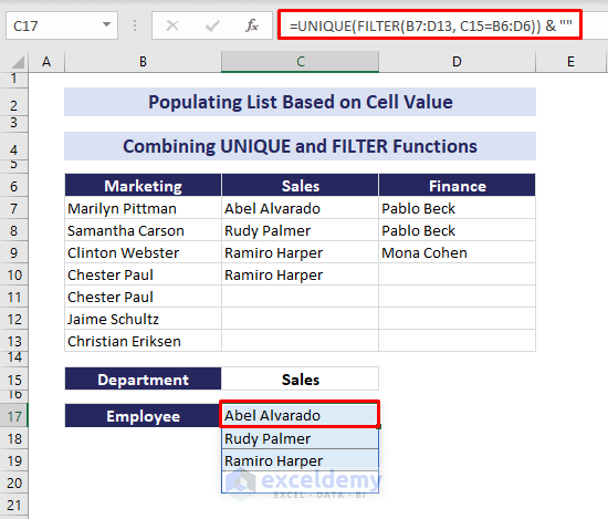
- Ramiro Harper was found twice in the Sales department in the main dataset. In the spilled result, the name occurs only once.
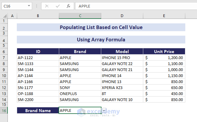
Method 5 – Populating a List Based on Cell Value by Using an Array Formula
In the following image, we have some IDs, Brands, Model names, and the Unit Prices of different mobile phones. We’ll select a brand name in cell C16 from the drop-down and want to get all the information about the mobile phones available for that brand only.
Steps:
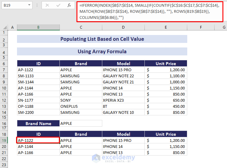
- Select cell B19.
- Insert the following formula:
=IFERROR(INDEX($B$7:$E$14,SMALL(IF(COUNTIF($C$16:$C$17,$C$7:$C$14), MATCH(ROW($B$7:$E$14), ROW($B$7:$E$14)), ""), ROWS(B19:$B$19)), COLUMNS($B$6:B6)),"")- Press Enter.
- Apply AutoFill to the right side and also to the cells below.
- You’ll get a list of all the information about the mobile phones for that brand only.
- You can change the cell formatting for the Unit Prices from General to Accounting through the Number group in the Home tab.
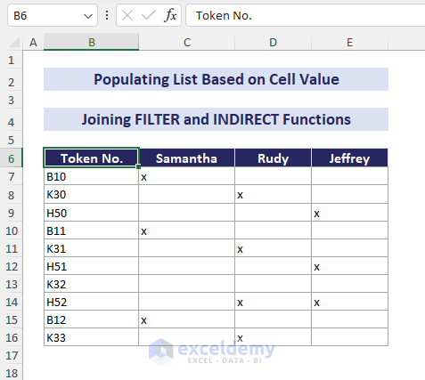
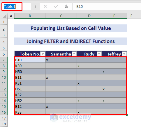
Method 6 – Joining the FILTER and INDIRECT Functions to Populate a List Based on Cell Value
Customers get a token based on the service they need whenever they go to a bank. Each of the bank employees provides a particular service, so different token types are assigned to different employees (denoted by x). We want to get the list of token numbers assigned to a particular employee we select.
Steps:
- Select the range B6:E16.
- Go to the Insert tab.
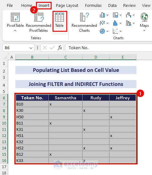
- In the Tables group, select Table.
- The Create Table dialog box will appear.
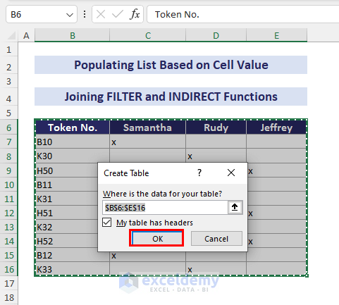
- Press OK.
- This will create an Excel table.
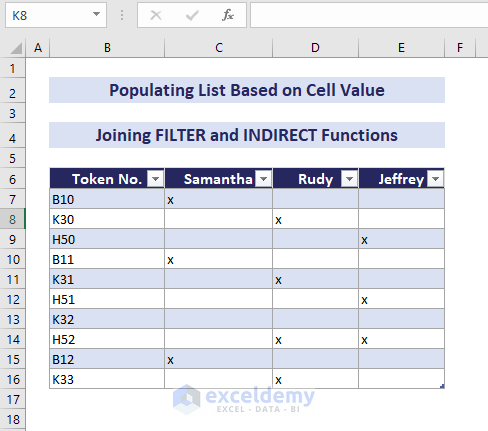
- Select the range B7:E16.
- Type Table1 in the Name Box to name the selected range.
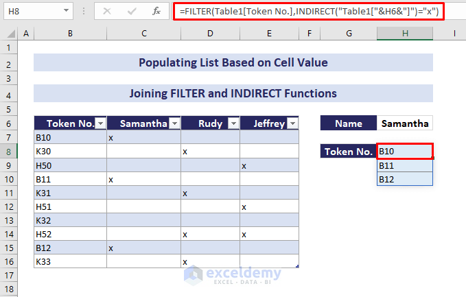
- Select cell H8.
- Insert the following formula:
=FILTER(Table1[Token No.],INDIRECT("Table1["&H6&"]")="x")- Press Enter. It’ll spill the list of token numbers assigned to the employee from cell H6.
Read More: Create Excel Filter Using Drop-Down List Based on Cell Value
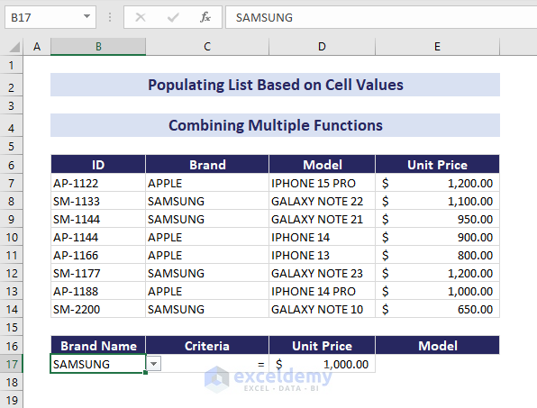
Method 7 – Populating a List Based on Multiple Cell Values in Excel
We have IDs, Brands, Model names, and Unit Prices of several mobile phones. We’ll populate a list of phones by Model names based on the Brand Name and the Unit Price.
Steps:
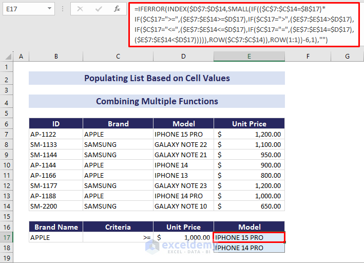
- Select cell E17.
- Insert the formula:
=IFERROR(INDEX($D$7:$D$14,SMALL(IF(($C$7:$C$14=$B$17)*IF($C$17=">=",($E$7:$E$14>=$D$17), IF($C$17=">",($E$7:$E$14>$D$17), IF($C$17="<=",($E$7:$E$14<=$D$17), IF($C$17="=",($E$7:$E$14=$D$17), ($E$7:$E$14<$D$17))))), ROW($C$7:$C$14)), ROW(1:1))-6,1),"")- Press Enter.
- Apply AutoFill.
The following GIF shows how to apply AutoFill.
Read More: How to Create Dependent Drop Down List with Multiple Words in Excel
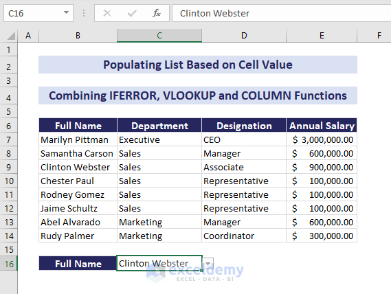
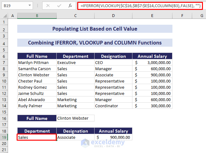
Method 8 – Combining IFERROR, VLOOKUP, and COLUMN Functions to Populate the List Based on Cell Value
We have the Full Name of the employees, their Department, Designation, and Annual Salary. We want to extract the list of info based on their Full Name. Since we have the names in the first column of the dataset, we can use the VLOOKUP function.
Steps:
- Select cell B19.
- Insert the following formula:
=IFERROR(VLOOKUP($C$16,$B$7:$E$14,COLUMN(B3),FALSE), "")- Press Enter.
- Drag the AutoFill icon to the right.
Download the Practice Workbook
Further Readings
- Conditional Drop Down List in Excel
- How to Make Dependent Drop Down List with Spaces in Excel
- How to Extract Data Based on a Drop Down List Selection in Excel
- How to Change Drop Down List Based on Cell Value in Excel
<< Go Back to Excel Drop-Down List | Data Validation in Excel | Learn Excel
Get FREE Advanced Excel Exercises with Solutions!

Thank you much for very useful tools Md. Abdullah!
I do have a question…
On solution #1 the list fill cell formula is :
=IFERROR(INDEX($B$4:$D$12,ROW(B3:D12),MATCH($C$14,$B$4:$D$4,0)),””)
There is no data on Row 3… why does formula use ROW(B3:D12)? Yet INDEX & MATCH use B4?
Just trying to understand how formula works better. Thanks!
Thank you ROB for your comment. Here, ROW function is working as the row index number of the INDEX function. Actually, it should be ROW(B2:D9)=> {2;3;4;5;6;7;8;9} which denotes respectively the 2nd, 3rd, 4th…. up to 9th row number of this ($B$4:$D$12) array of INDEX function. Here, we ignore the 1st row of ($B$4:$D$12) this array as 1st row contains the Club Name’s not any player Name’s.
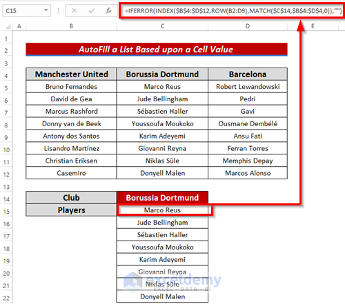
On the other hand, you have to use B4:D4 row in the MATCH function which will search for the Club Name’s and act as the column index number in the INDEX function.
Say, when you choose Borussia Dortmund or C4 cell from the list of C14 cell then the MATCH function will return 2 and thus the column index number of INDEX function will be 2 so INDEX function will give all the rows (except 1st one) of 2nd column of the given array which means all the player name’s of the Borussia Dortmund club.
So, you can use the formula like the below one. =IFERROR(INDEX($B$4:$D$12,ROW(B2:D9),MATCH($C$14,$B$4:$D$4,0)),””)
Can someone please help me understand what I need to do? I have column A,B,C. A and B have a persons first name and surname, C is a Yes or no answer indicated by Y or N.
I want a formula that will copy their name into another sheet but only if the answer in C is Y.
Thanks for reaching out.
You can follow method 3 of this article to accomplish your task. Go to the destination sheet and click a cell where you want to paste the names. Insert this formula:
=FILTER(Source!A2:B20, “Y”=Source!C2:C20)
Press Enter to get the results. Here, “Source” is the sheet name of your source sheet where the names are present along with Yes/No. A2:B20 is the cell range of the first and last names. Change it according to your dataset. C2:C20 is the cell range with Yes/No.
This should work. Hope this helped.
Regards,
Aung
ExcelDemy.
Hi
so, I have tried to follow each of the steps outlined and they are so clear and concise I hate to ask my question, but I keep getting stuck – so apologies first and foremost.
I have 4 columns of data let’s say – Subs / Employee / Title / Rate
Depending on which Sub is selected then the associated list of employees for that Sub should be selectable in the employee column and likewise their Title and rate should reflect in the next columns – no matter what I do I cannot get them to align
Any ideas would be MUCH appreciated
Hello BEN
Thanks for reaching out and sharing your problem. The requirements you mentioned can be achieved by following some steps.
Follow these steps:
Step 1: Create a Drop-down for Subs
Step 2: Find Employees Based on Subs in an Intermediate Column
Select cell F2 => Insert the following formula => Hit Enter.
Step 3: Create a Drop-down for Employees
Step 4: Display Title and Rate Based on Employee
Select cell C23 => Insert the following formula => Hit Enter.
Step 5: Hide the Intermediate Column and Insert an Event Procedure
Hide column F => Right-click on the sheet name tab => Click on View Code => Paste the following code in the sheet module => Save.
OUTPUT: Return to the sheet and make desired changes to see the result like the following GIF.
You can download the solution workbook for better understanding.
Download Solution Workbook
Hopefully, the idea will help you in reaching your goal. Good luck!
Regards
Lutfor Rahman Shimanto