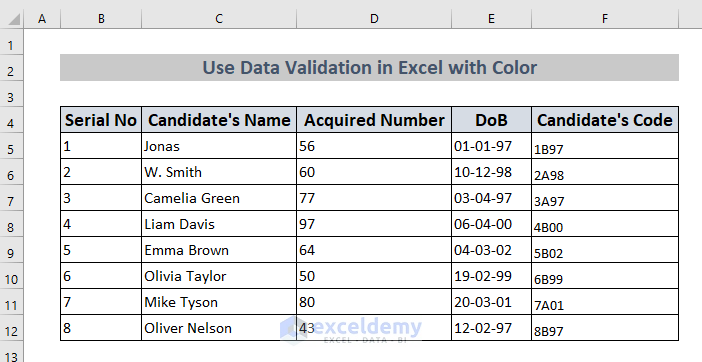
How to Use Data Validation in Excel with Color (4 Ways)

We have a dataset containing five columns: Serial Number, Candidate Name, Acquired Number, DoB, and Candidate’s Code. We will use different Columns of our dataset to demonstrate different methods for using Data Validation in Excel with color.

Method 1 – Using Whole Numbers for Data Validation in Excel with Color

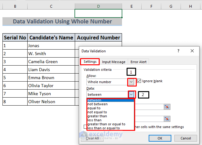
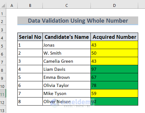
The Acquired Number Column is blank which we will now fill by applying Data Validation. We want to put the condition that only numbers between 40 and 100 can be given as input.

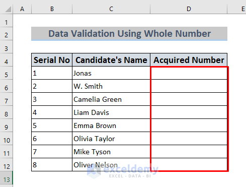
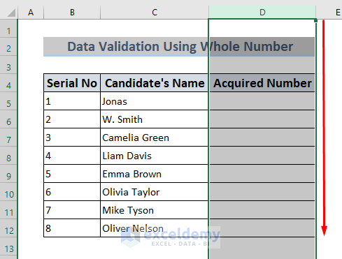
Select the column where we will apply Data Validation. We have selected the Acquired Number column.

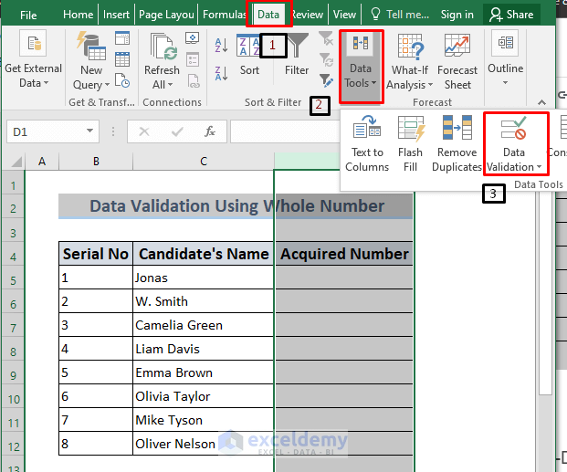
Go to the Data tab, select Data Tools, and choose Data Validation.

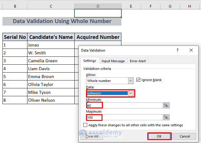
The Data Validation window will open. Click the Allow box and select Whole number.
In the Data box, select Between.

Put 40 in Minimum and 100 in Maximum.
Click OK.

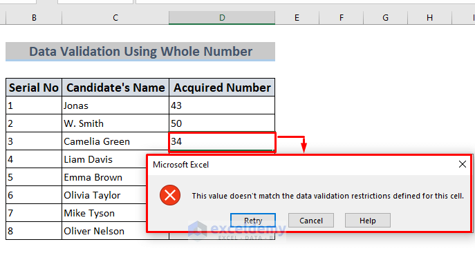
Enter the values manually.
If you try to enter any number less than 40 or more than 100, Excel will show an error message.

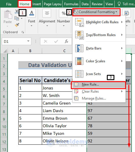
Let’s put numbers from 40 to 59 in yellow and 60 to 100 in green.

Select the column.
Go to Conditional Formatting and select New Rule.

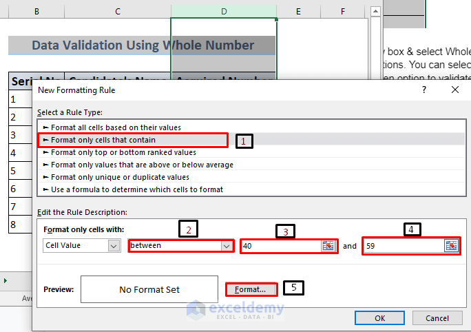
Select Format only cells that contain.
Go to the Edit the rule description part.
The first box will be Cell Value. Keep it as is for the sample.
In the next box, put between. Type 40 and 59 in the following two boxes as the limiting values.
Click Format.

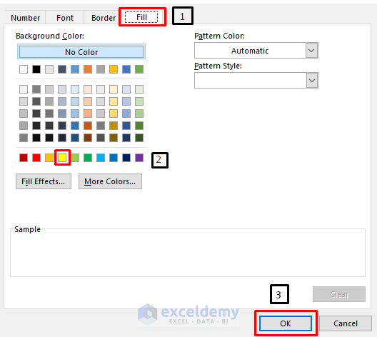
Choose a yellow color from the Fill tab and click OK.

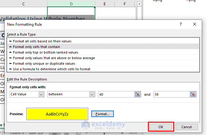
Click OK again on the first dialog box.

All the cells of the Acquired Number column with values between 40 and 59 will be colored yellow.

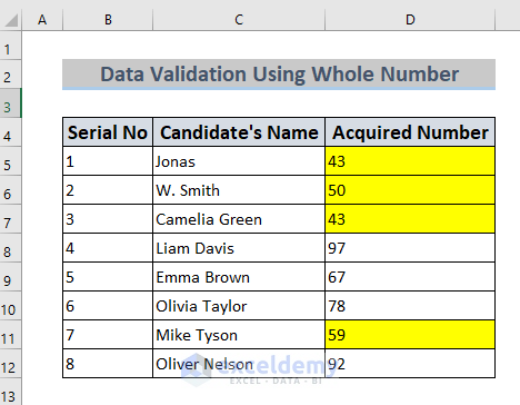
Repeat the same process for the second formatting rule, with limits between 60 and 100 and a green fill.

Method 2 – Creating a Drop-Down List with Color Using Excel Data Validation

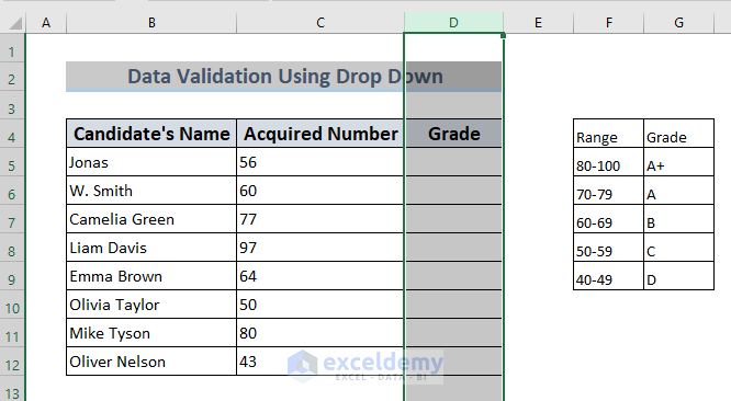
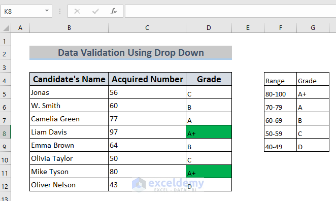
Suppose we have a dataset like the previous one with an additional Grade column where we want to input the grade depending on the number range.

Put the scoring table next to the dataset.
Select the Grade column.

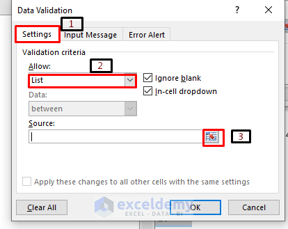
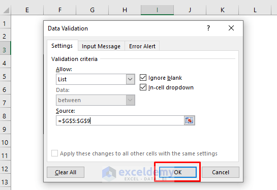
Open the Data Validation dialog box and select List in Allow.
Click on the icon on the far right of the Source box to add the source.

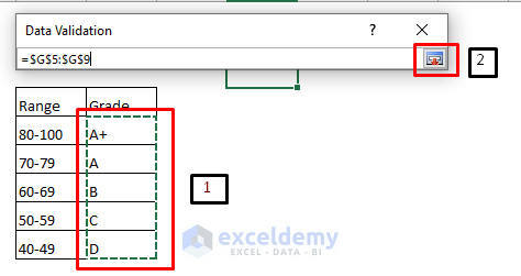
Select the scoring table’s grade column.
Click on the Source button again.

Click OK in the Data Validation dialogue box.

You will get a drop-down menu in every cell of the Grade column.
Enter a grade for each cell via the drop-downs.

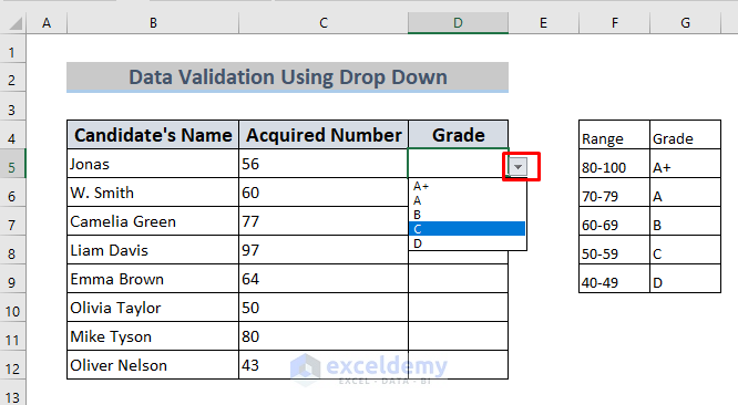
Here is what we did for the sample.

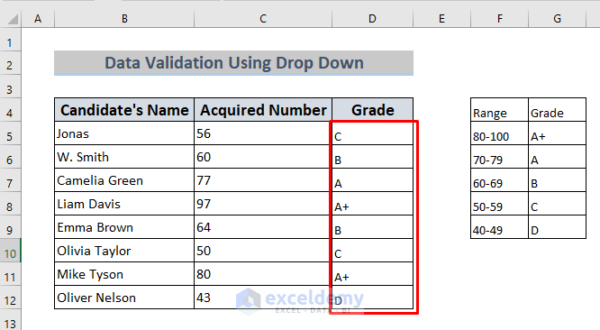
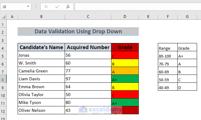
We want to have different colors for different Grades.

Open Conditional Formatting.
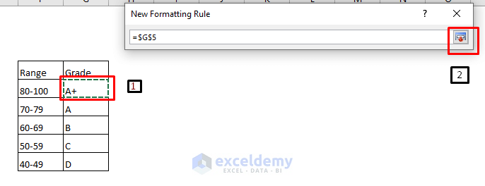
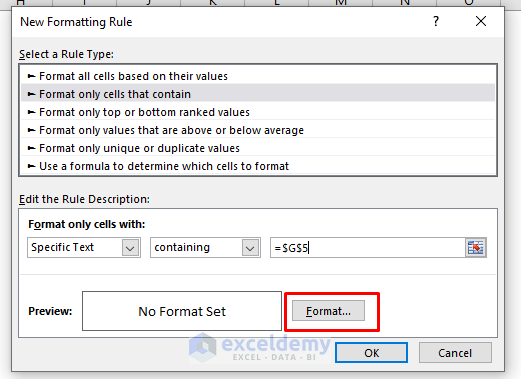
Select Specific Text in the first box, Containing in the second, and click on the Source selector icon.

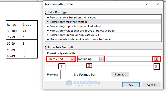
Select the A+ cell from the scoring table and click on the selector.

Click on Format.

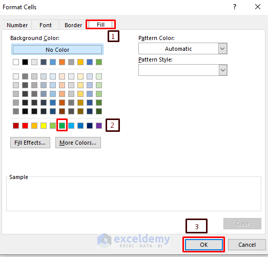
Choose the desired color in Fill and click on OK.

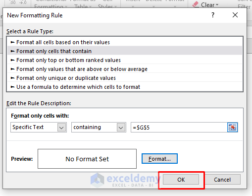
Press OK in the Conditional Formatting dialogue box.

We chose a green color for A+.

Repeat the process for each other grade, selecting a different fill color each time.

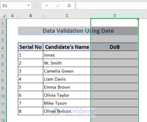
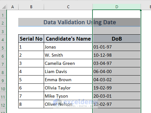
Method 3 – Selecting a Date with Color with Data Validation in Excel

Steps:

We want to sort out candidates depending on their date of birth, where only candidates born between 01-01-1997 and 01-01-2003 are eligible.

Select the DoB column.

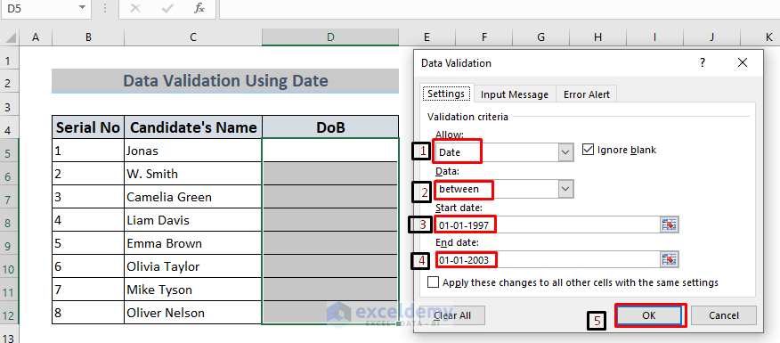
Open Data Validation.
In Allow, put Date.
For Data, put between.
Enter the Start date and the End date.
Click OK.

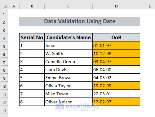
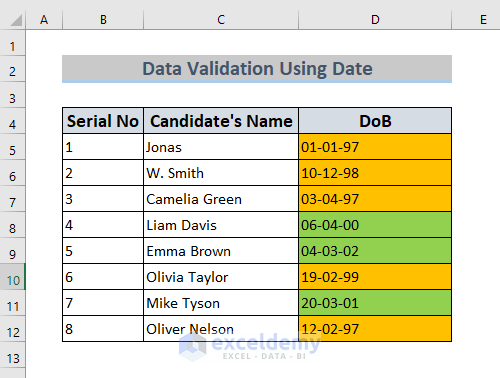
Candidates born between 01-01-1997 and 31-12-1999 will be marked orange and candidates born between 01-01-2000 and 01-01-2003 will be marked green.

Select the DoB Column.

Go to New Formatting Rule.
Choose Cell Value, then between.
Enter the starting and ending date for the category and click Format.

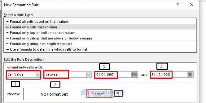
Choose a fill color and click OK twice to apply.

Repeat the process for every category you want.

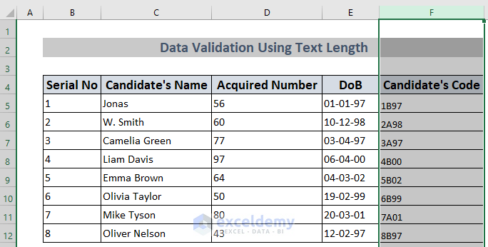
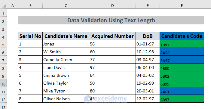
Method 4 – Applying Data Validation for Selecting Text Length with Color

Steps:

Suppose we have a dataset with Candidate’s Code in Column F. It’s tough to type the code manually since they don’t have any direct correlation to other values. We will restrict the length of the value with Data Validation.

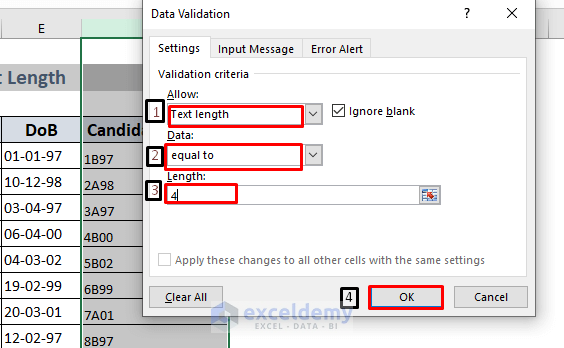
Select the Candidate’s Code column.

Go to Data Validation.
For Allow, put Text Length.
Choose equal to for Data
Enter 4 (desired character length) in the Length box.
Click OK.

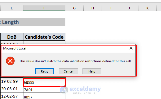
If the input is shorter or longer, Excel will show a warning message.

We can color the cells based on the letter in the code.

Select the Candidate’s Code column again.

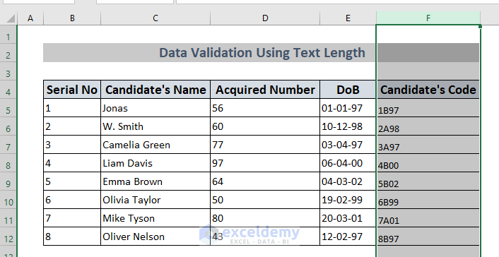
Following the procedures shown in Method 3, choose Specific Value and enter the character you want to format with (in this case A for one and B for the other).
Choose a color for each category.
Repeat the process to make the second category. Here’s our sample result.