Finding matches is an integral part of data analysis. From searching out relevant information from a large dataset to finding errors by matching values, the possibilities of the MATCH function are endless. We can use it in conditional formatting too for matching specific criteria. Also, we can use it with other functions like INDEX or VLOOKUP to create useful combinations.
Download the Practice Workbook
What Is the MATCH Function in Excel?
The MATCH function locates a value within a range of cells and returns its position.
Syntax:
- lookup_value: The value you want to find.
- lookup_array: The range of cells to search in.
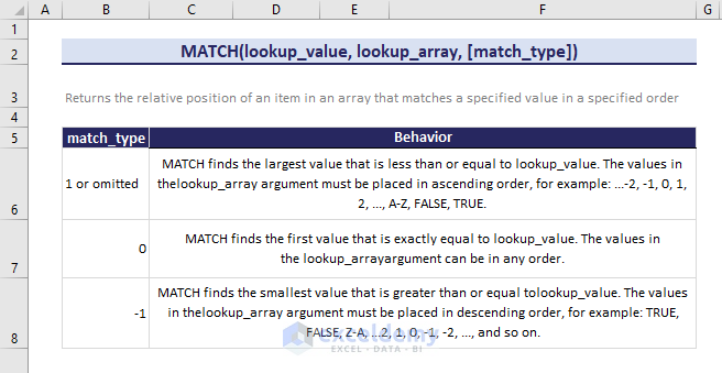
- match_type: The type of match to perform (0 for exact match, 1 for less than or equal to, -1 for greater than or equal to).
Example: =MATCH(“John”, A1:A5, 0) This formula searches for “John” in cells A1 to A5 and returns the position of the value if found.
Related Functions:
Click on the functions individually to learn more about various match functions in Excel.
How to Find a Match in Excel?
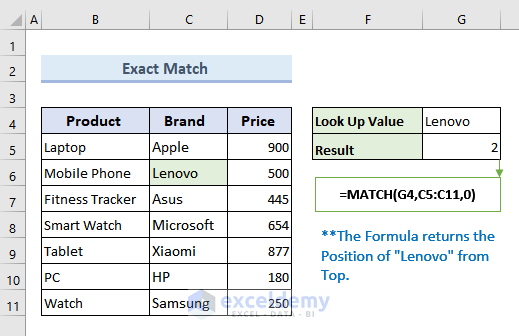
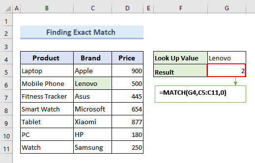
Case 1 – Find an Exact Match
We need to use zero as the third argument to find the exact match using the MATCH function.
- Select cell G5 and use the formula.
=MATCH(G4,C5:C11,0)- Press Enter.
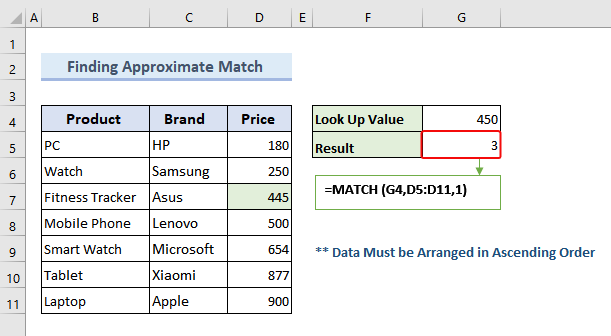
Case 2 – Find an Approximate Match
- Arrange the column that contains the search array in ascending order.
- In cell G5, use the formula below and press Enter.
=MATCH(G4,D5:D11,1)This will return the position of the data. If the column is not sorted by ascending order, MATCH will find the first value larger than the search term and return the location before it, even if there’s a closer match down the array.
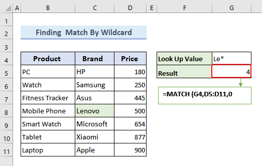
Case 3 – Use a Wildcard Match to Search with a Partial Value
Let’s search for Lenovo in the dataset by just using Len* as a lookup value.
- Use the formula below in cell G5 and press Enter.
=MATCH(G4,C5:C11,0)This should return the relative position 4 in the “Brand” Column.
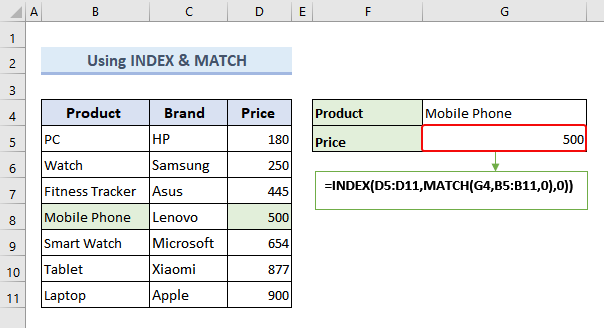
Case 4 – Use the INDEX and MATCH Functions to Find a Value Based on a Condition
- Select G5 and use the formula below.
=INDEX(D5:D11,MATCH(G4,B5:B11,0),0)- Press Enter.
The price of the “Mobile Phone” option should come in cell G6 as shown in the figure.
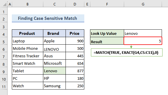
Case 5 – Perform a Case-sensitive Match
- In cell G5, use the following formula and press Enter.
=MATCH(TRUE, EXACT(G4,C5:C11),0)It will return the column index number of “Lenovo” but not “LENOVO”.
Read More: Match Names in Excel Where Spelling Differ
Case 6 – Compare Two Columns for Matches and Differences
We will find matching values in two columns and compare them. If values of Product List-2 are present in Product List-1, it will return Blank. Otherwise, it will return “Not in List 1”.
- Select cell D5 and enter this formula for a Case-Insensitive Search.
=IF(ISNA(MATCH(C5,$B$5:$B$11,0)), "Not in List 1", "")- For case-sensitive searches, use this formula in cell E5.
=IF(ISNA(MATCH(TRUE, EXACT(B:B, C5),0)), "Not in List 1", "")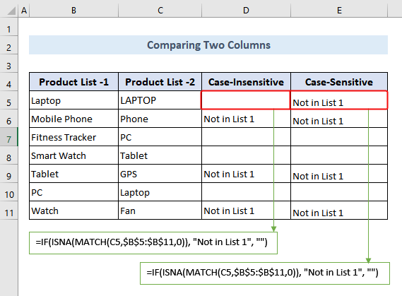
Read More: Return the Row Number of a Cell Match in Excel
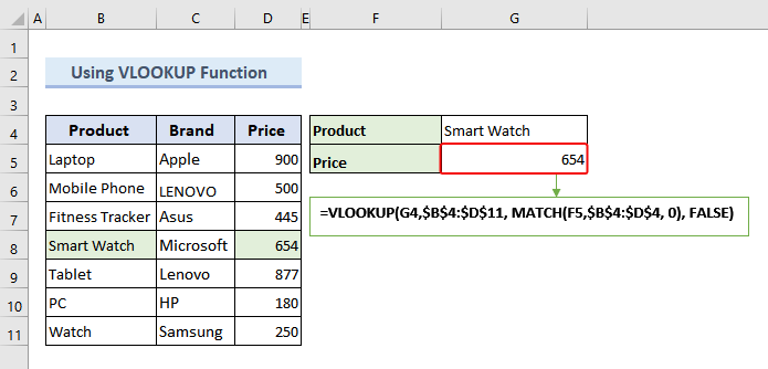
Case 7 – Use VLOOKUP and MATCH to Find a Specific Value
- Select cell G5 and insert the following formula.
=VLOOKUP(G4,$B$4:$D$11, MATCH(F5,$B$4:$D$4, 0), FALSE)- Press the Enter button.
This will return the Price of “Smart Watch,” which is 654.
Read More: If One Cell Equals Another Then Return Another Cell in Excel
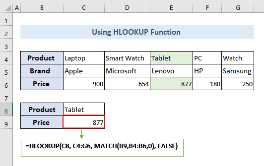
Case 8 – Combine HLOOKUP and MATCH Functions to Search for a Particular Value
- In cell C9, use the following formula and press Enter.
=HLOOKUP(C8, C4:G6, MATCH(B9,B4:B6,0), FALSE)It will return the Price of the Tablet from the dataset.
Things to Remember
- The MATCH function in Excel is designed to return the position of the first matching value found within the specified range. If the range contains multiple occurrences of the lookup value, the MATCH function will only return the position of the first match it encounters.
- For the approximate match, the range must be sorted in ascending order.
- Use error handling functions like IFERROR or ISNA to manage errors.
- Ensure the range contains the desired values.
Frequently Asked Questions
How do you use Match in Excel?
To use the MATCH function in Excel, designate the result cell, input “=MATCH(” in it, and provide the value you’re seeking and the search range. You can include a third argument for match type (0, 1, or -1). Conclude the formula with “)” and press Enter to find the value’s position within the range.
For example, if you want to find the position of the value “5” in the range A1:A10, you would enter “=MATCH (5, A1:A10, 0)“.
What is INDEX MATCH in Excel?
INDEX-MATCH is a powerful combination of Excel functions. It allows you to find a value in one column (MATCH) and retrieve a corresponding value from another column (INDEX). It’s more flexible than VLOOKUP and HLOOKUP, making it ideal for complex lookups and large datasets.
What is the exact match command in Excel?
The “exact match” command in Excel means using the option that ensures the lookup value matches exactly with the data being searched. It avoids any partial or approximate matches, providing precise results.
Excel Match: Knowledge Hub
<< Go Back to | Learn Excel
Get FREE Advanced Excel Exercises with Solutions!
