How to Match Data in Excel from 2 Worksheets (6 Methods)

Method 1 – Compare and Match Data from 2 Worksheets by Viewing Side-by-Side in Different Workbooks

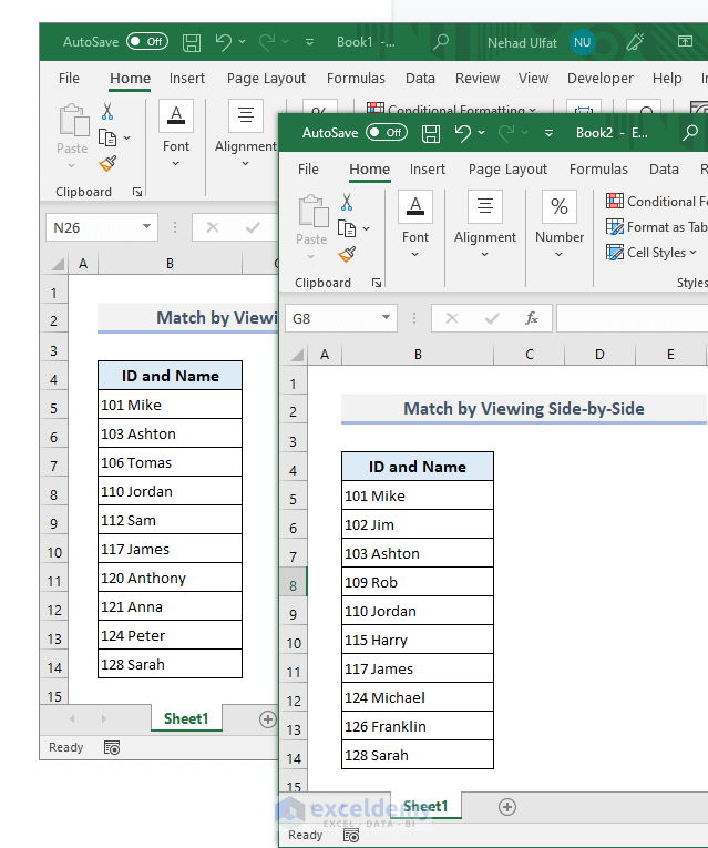
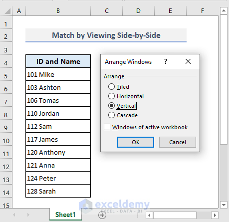
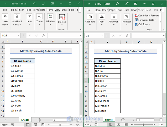
There are two sample workbooks named Book 1 and Book 2. Both workbooks contain different datasets starting in the same cell in Column B.

We can display these workbooks side-by-side and compare data visually for matches.

 Steps:

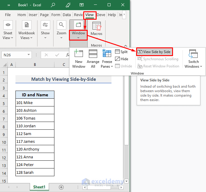
• Go to the first workbook Book 1.
• Under the View tab, select the View Side by Side command from the Window drop-down.

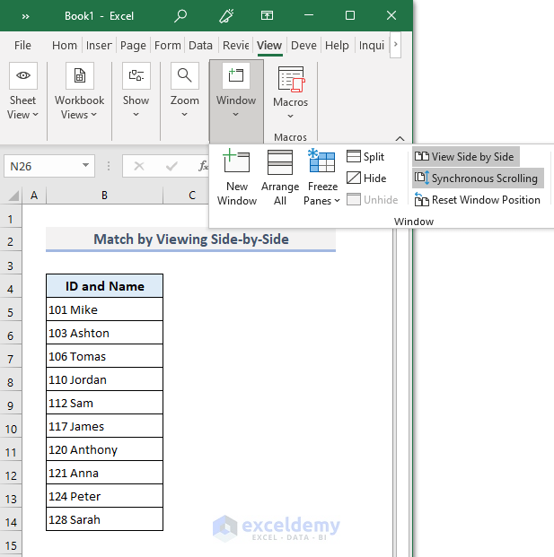
• Select Synchronous Scrolling under the View Side by Side option.

• Click on the Arrange All option. A dialog box will appear.

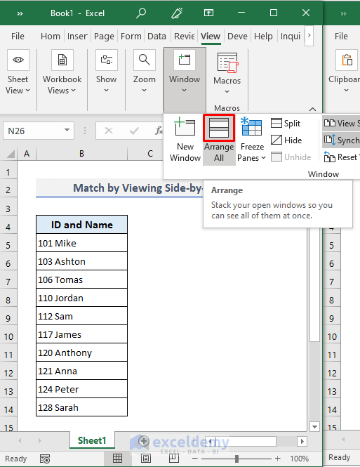
• Choose the Vertical radio button from the options and press OK.

The two workbooks are now displayed side-by-side for comparison. This method is helpful to compare a small amount of data visually and find matches side-by-side from two workbooks.

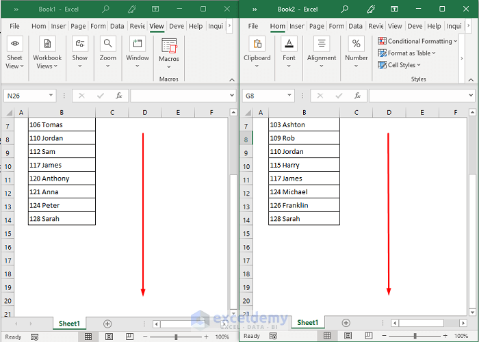
As we’ve enabled Synchronous Scrolling, so if we scroll down in a workbook the other workbook will follow.

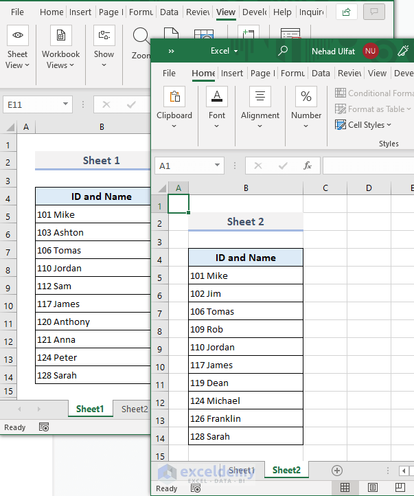
Method 2 – Compare and Match Data from 2 Worksheets by Viewing Side-by-Side in separate Workbook

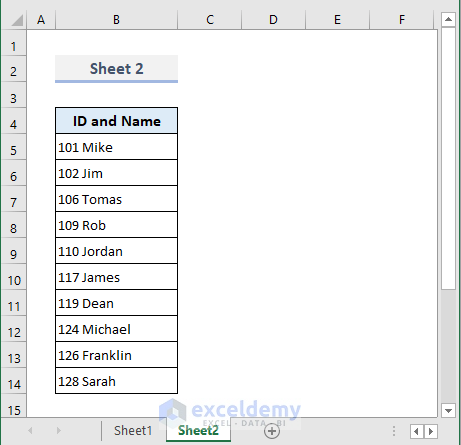
In this example there are two worksheets named Sheet1 and Sheet2 within a single Excel workbook.

Steps:

• Go to the View ribbon.
• From the Window dropdown, select New Window.

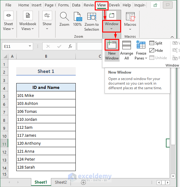
• The sheets are now displayed as two different workbooks as shown in the following picture.
• Repeat the steps in the first method to compare data for Sheet1 from the first workbook and Sheet2 from the second workbook and find matches visually.

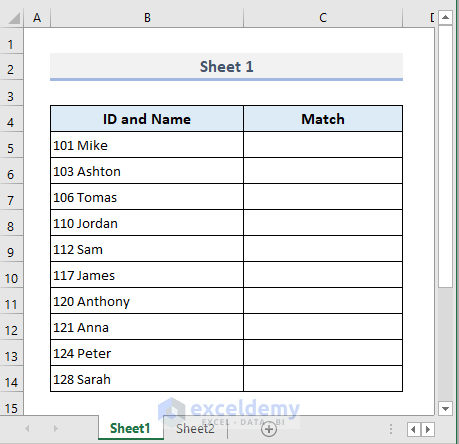
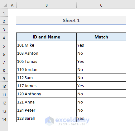
Method 3 – Match Data Side-by-Side from 2 Worksheets in Same Workbook and Return Outputs in Excel

The IF function will return the message Yes for the matched data and No for the non-matches.

Steps:

• In cell C5 in Sheet1, enter the following formula:

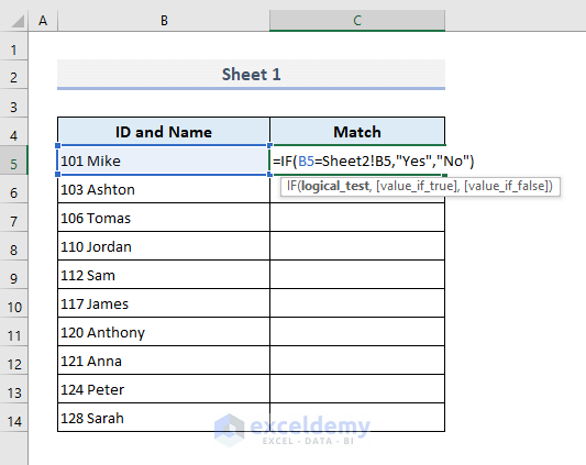
• Press Enter and use Fill Handle to autofill the rest of the cells in Column C under the Match header.

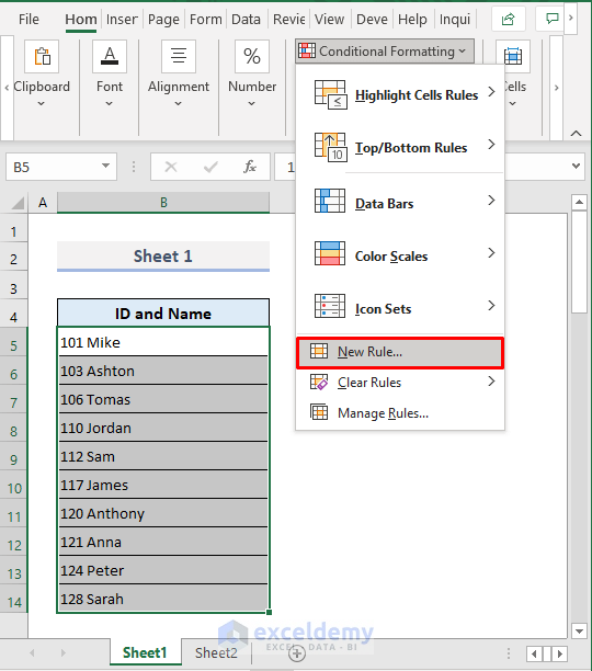
Method 4 – Match Data Side-by-Side from 2 Worksheets in Excel with Conditional Formatting

Steps:

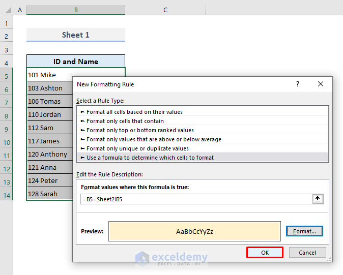
• Under the Home tab, select the option New Rule from the Conditional Formatting dropdown.
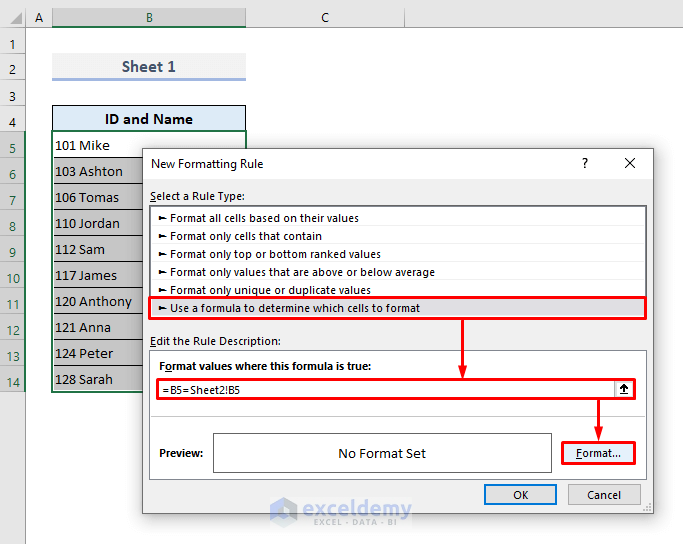
• A dialog box named New Formatting Rule will appear.

• Select the option Use a formula to determine which cells to format.
• In the Rule Description box, enter the following formula:

• Press Format.

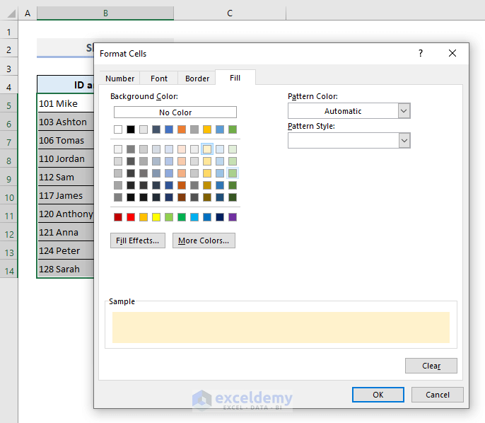
• In the Format Cells window, select the Fill tab.
• Select a color that will highlight the matches from two worksheets.
• Press OK.

• The New Formatting Rule dialog box will display a preview of the highlighted cell with text at the bottom.
• Press OK.

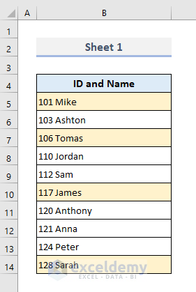
In Sheet1, the matches are highlighted with the specified color.

Method 5 – Use VLOOKUP to Match Data from 2 Worksheets and Return Values in Excel

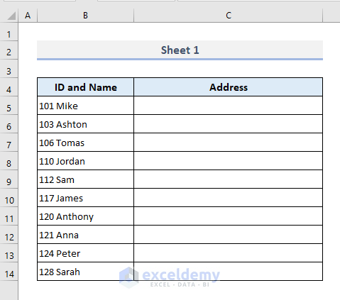
The first sheet contains a table with ID and Name and Address headers.

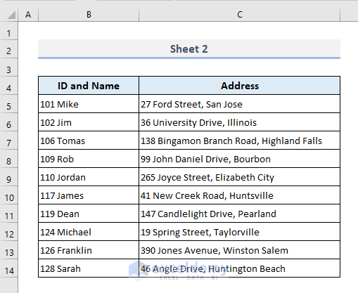
The second worksheet contains the complete dataset.

VLOOKUP can be used to find matches in the second worksheet (Sheet2), extract addresses for the corresponding matches, and display them in the first worksheet (Sheet1).

As the VLOOKUP function will return a #N/A error if a match is not found, we’ll combine the VLOOKUP function with the IFERROR function.

This will return a customized message Not Found if the VLOOKUP function does not find a match in Sheet2.

Steps:

• Enter the below formula in cell C5 of Sheet1:

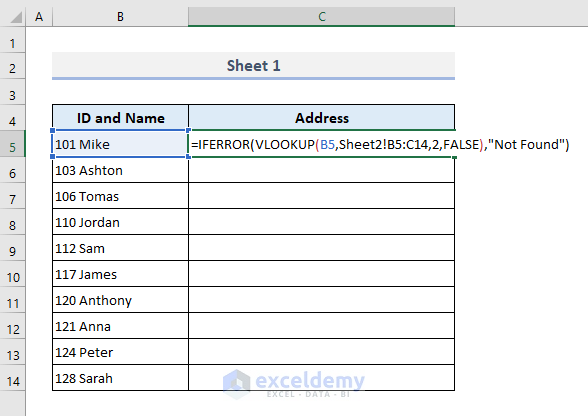
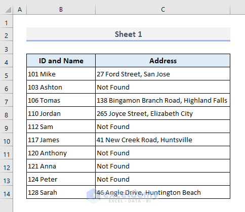
• Fill the entire column using the fill handle to return the following outputs under the Address header in Sheet1.

Method 6 – Apply INDEX-MATCH Formula to Match Data and Return Values after Comparing 2 Worksheets

The INDEX function returns a value or reference from a cell in a given range, and the MATCH function returns the relative position of an item in an array that matches a specified value in a specified order.

Since the INDEX-MATCH formula will return an error if a match is not found, we’ll again use the IFERROR function to customize a return message for the non-matches.

Steps:

• Enter the below formula in cell C5:

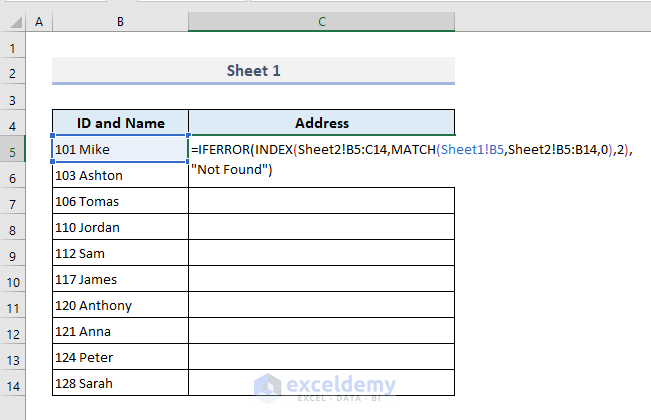
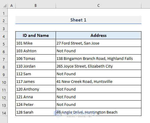
• Press Enter and autofill the rest of the cells in Column C.

Download Practice Workbook

<< Go Back to | Excel Match | Learn Excel