Excel Find Matching Values in Two Columns

Method 1 – Find Matching Values in Two Columns Using the IF Function

We have two lists of fruit names and want to find matching fruit names between List 1 and List 2.

Steps:

• Use the following formula in cell D5.

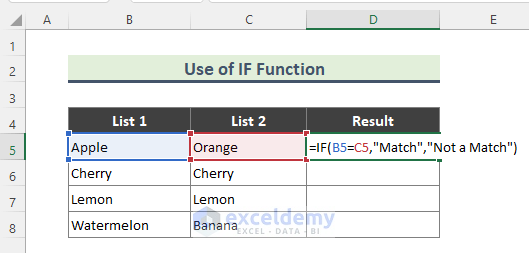
The IF function checks whether a condition is met, and returns the value if TRUE, and another value if FALSE.

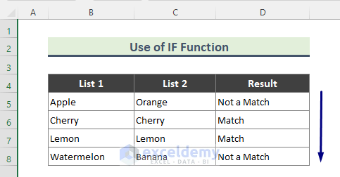
• Use the Fill handle (+) tool to copy the formula to the rest of the cells.

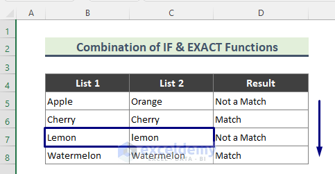
Method 2 – Combination of IF and EXACT functions to Get Matching Values in Two Columns (Case Sensitive)

Steps:

• Insert the following formula in cell D5.

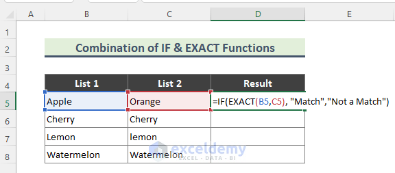
• Use AutoFill.

Method 3 – Excel IF, AND/OR Combination to Find Matching Values in Two Columns

Steps:

• Use the following formula in cell D5.

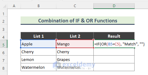
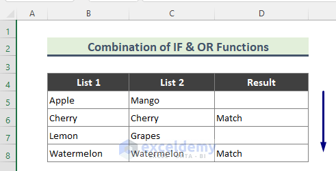
• Here is the output according to the typed formula.

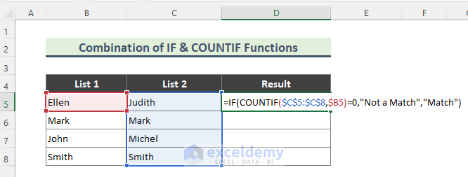
Method 4 – Find Matching Values in Two Columns Excel with a Combination of IF and COUNTIF Functions

We have two lists of people’s names and want to find whether names from one list appear in the other.

Steps:

• Use the following formula:

This formula checks whether the value in B5 matches any values in column C5:C8.

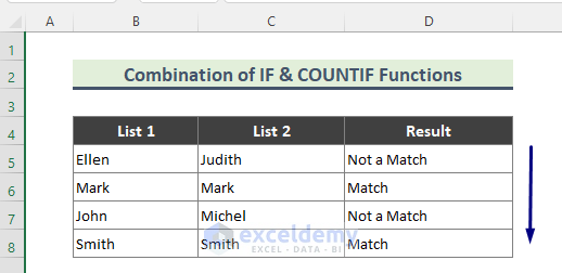
• AutoFill the formula down.

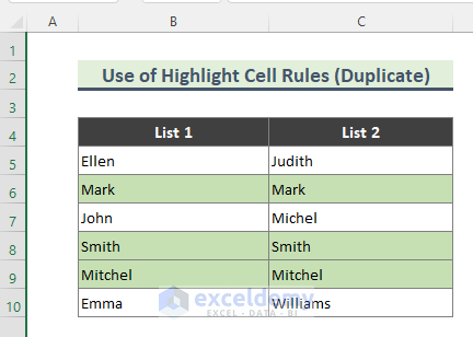
Method 5 – Use Highlight Cell Rules to Find Matching Values in Two Columns in Excel

Steps:

• Select the entire dataset (B5:C10).

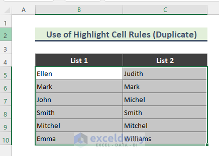
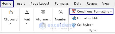
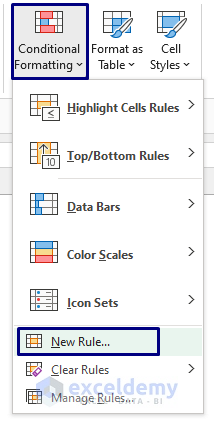
• Go to Home and select Conditional Formatting.

• Go to Highlight Cell Rules and choose Duplicate Values.

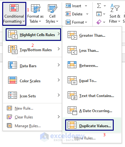
• The Duplicate Values window will show up.
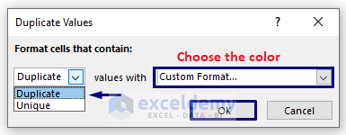
• Select the Duplicate option from the drop-down.
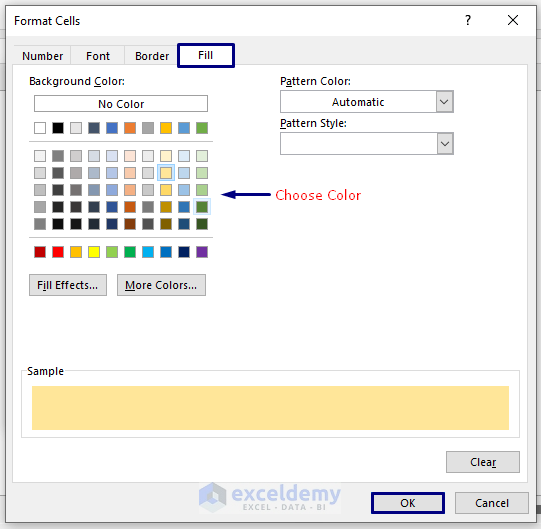
• Choose the highlight color or you can choose the color from Custom Format.
• Click OK.

• Values that appear twice or more through the dataset will be highlighted.

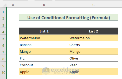
Method 6 – Get Matching Values in Two Columns Using Conditional Formatting (Arithmetic Formula)

Steps:

• Select the entire dataset (B5:C10).

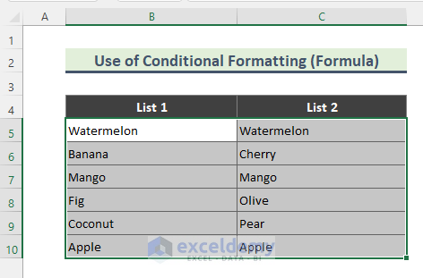
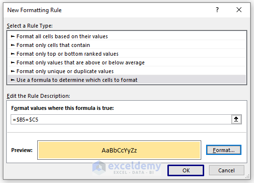
• Go to Home, then to Conditional Formatting, and select New Rule.

• The New Formatting Rule window will show up.
• Choose the Use a formula to determine which cells to format option.
• Use the following formula in the Format values where this formula is true: field.

• Click on Format.

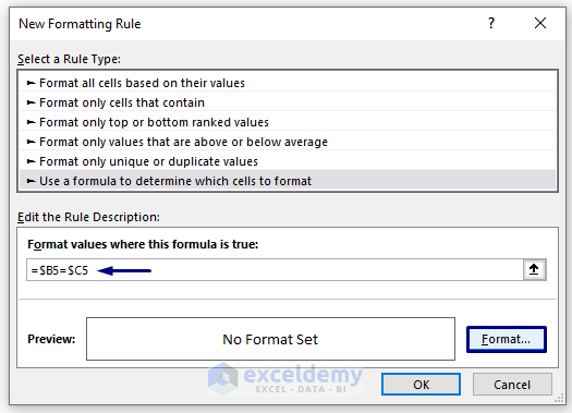
• Click the Fill tab, choose the highlight color, and click OK.

• Click OK.

• Matched fruit names will be highlighted.

Method 7 – Apply IFERROR and VLOOKUP to Search Matching Values in Two Columns in Excel

Steps:

• Use the following formula in cell C5.

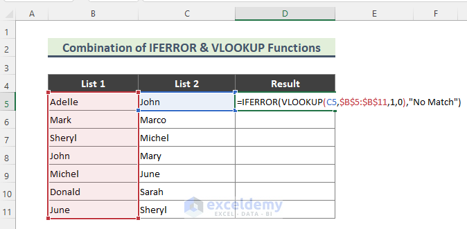
• Use AutoFill.

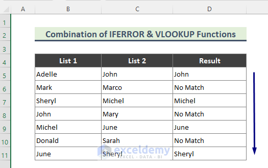
Breakdown of the Formula:

VLOOKUP(C5,$B$5:$B$11,1,0)

The VLOOKUP function looks for a value in the leftmost column of a table and then returns a value in the same row from a column you specify.  So, the function will look for C5 in the range B5:B11 and return:

{John}

Conversely, when the function finds C6 to range B5:B11, it will return a #N/A error because C6 is not present in the prescribed range.

IFERROR(VLOOKUP(C5,$B$5:$B$11,1,0),”No Match”)

The IFERROR function returns value_if_error if the expression is an error and the value of the expression itself otherwise. In our example, we have put No Match as an argument. As a result, when we will look for C6 in the above-mentioned range, the formula returns:

{No Match}

Method 8 – Search Matching Values with a Combination of INDEX and MATCH Functions in Excel

We have two tables that have a common column Fruit Name. We will match the tables by that column and return the quantity from the first table into the second one.

Steps:

• Insert the following formula in cell F5.

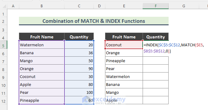
• Use AutoFill.

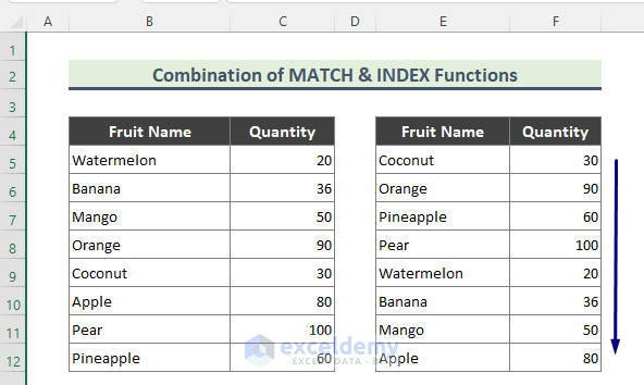
Breakdown of the Formula:

MATCH($E5,$B$5:$B$12,0)

The MATCH function returns the relative position of the value of cell E5 in the array (B5:B12)  that matches a specified value in a specified order.

INDEX($C$5:$C$12,MATCH($E5,$B$5:$B$12,0))

The INDEX function returns a value or reference of the cell at the intersection of a particular row and column, in a given range (C5:C12) and thus replying the Quantity of the fruit accordingly.

Download the Practice Workbook

<< Go Back to | Excel Match | Learn Excel