Compare Two Lists in Excel for Matches (All Methods and Uses)

Here’s an overview of comparing two lists for matches with an exact match via IF.

How to Compare Two Lists for Matches in Excel

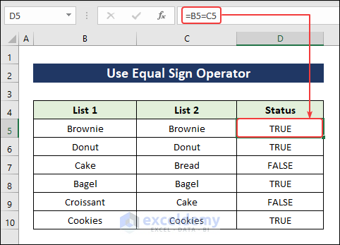
Method 1 – Using the Equal Sign Operator

This method finds matches in the same row.

• Select cell D5 and enter the following formula.

If cell B5 has the same data as cell C5, the result will be TRUE, otherwise, it will be FALSE.

• AutoFill the rest of Column D.

Method 2 – Applying Conditional Formatting

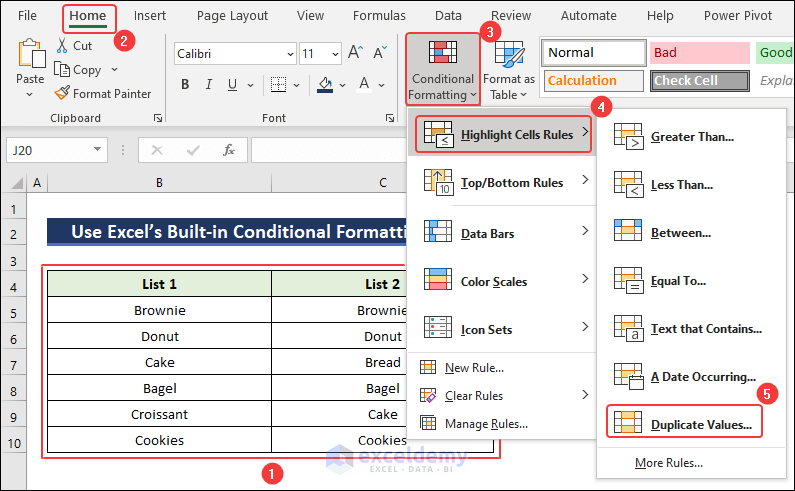
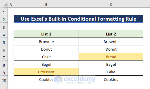
Case 2.1 – Using Excel’s Built-in Conditional Formatting Rule

We will highlight values that are present only once in two lists.

• Select both lists.
• Go to Conditional Formatting, select Highlight Cells Rules, then select Duplicate Values.

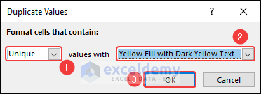
• In the Duplicate Values box, select Unique values and choose Yellow Fill with Dark Yellow Text, then click on the OK button.

• The cells with unique values will be highlighted.

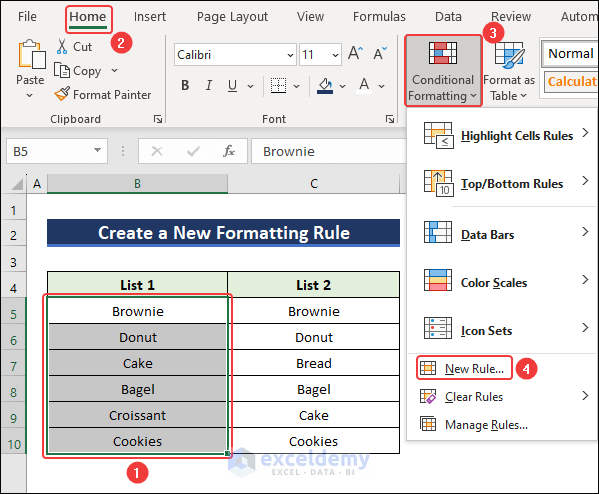
Case 2.2 – Creating a New Formatting Rule

• Select List 1 and go to Home, then select Conditional Formatting and pick New Rule.

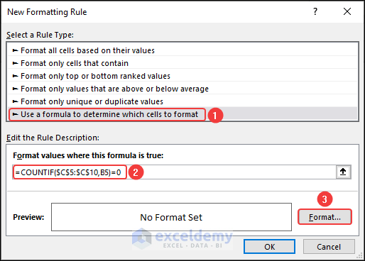
• Select Use a formula to determine which Cells to format and insert the following formula in Edit the Rule Description.

• Click on Format.

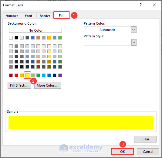
• Go to the Fill tab and change the fill color to yellow and click on the OK button.

• The values in List 1 that don’t exist in List 2 will be highlighted.

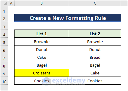
• You can repeat the process for List 2, inverting the formula.

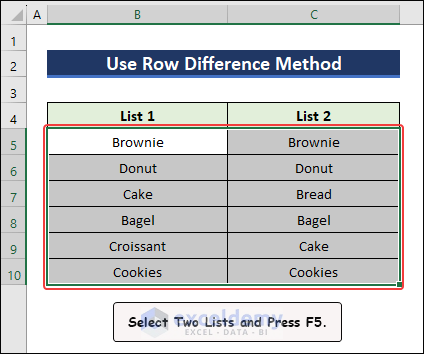
Method 3 – Using the Row Difference Option in Go To Special

• Select both lists and press F5 to open the Go To dialog box.

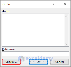
• Click on Special.

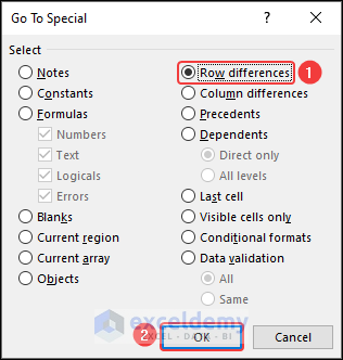
• Select Row differences and click OK.

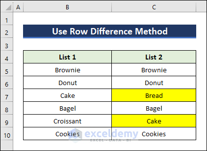
• The cells in List 2 that have different data will be selected.
• Go to the Home tab, choose the Fill Color tool, then select the Yellow color from Standard Colors group.

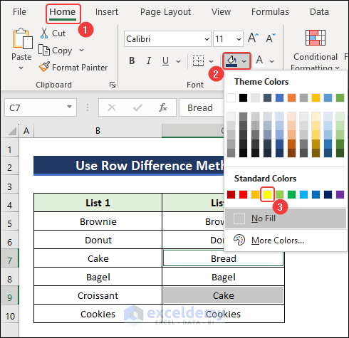
• This highlights the cells.

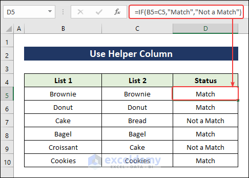
Method 4 – Using a Helper Column

• Add a third column named Status.
• Apply the following formula in the first cell of this column.

The rows having the same data will show Match as output, otherwise, it will return Not a Match.

• Use AutoFill.

Method 5 – Inserting the VLOOKUP Function

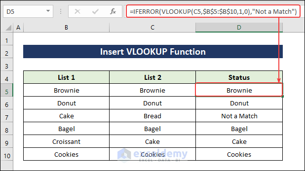
Case 5.1 – Finding a Full Match

• Select cell D5 and enter the formula given below.

If the data in List 2 is found in List 1, the output will be that data. If it is not found, the formula will return Not a Match.

• Use AutoFill.

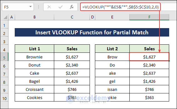
Case 5.2 – Finding a Partial Match

• Apply the following formula in cell F5.

This formula will return the Sales value using the partial matches of List 2.

• Use AutoFill.

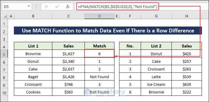
Method 6 – Using the MATCH Function to Match Data Even If There Is a Row Difference

• Select cell D5 and insert the following formula.

It will return the number of rows where it finds a match. Otherwise, it will return Not Found.

• Use AutoFill.

How to Compare Multiple Columns in Excel

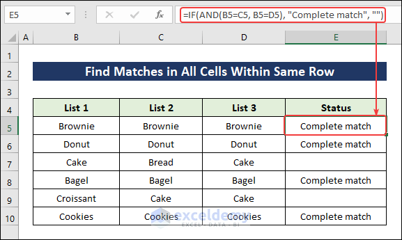
Method 1 – Find Matches in All Cells Within the Same Row

• Click on cell E5 and insert this formula.

If all three columns in the same row have the same data, the result will be a Complete match.

• Use AutoFill.

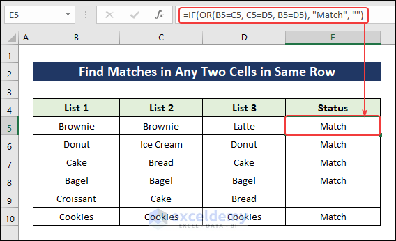
Method 2 – Find Matches in Any Two Cells in Same Row

• Select cell E5 and insert the following formula.

The output will be Match if any two of the three columns of the same row contain the same data.

• Use AutoFill.

Things to Remember

• If the lists are not organized, using row-by-row matching methods will not work.
• The Row Difference method only highlights the cells in List 2.

Frequently Asked Questions

Can I compare more than two lists simultaneously in Excel?

You can apply the Array formula or use Power Query to compare multiple lists simultaneously.

Is it possible to compare lists from different worksheets or workbooks?

You need to list the sheet or book reference before the cell reference. While using any formula to compare lists, you need to make sure to insert the correct worksheets and workbook references.

What are some common scenarios where comparing two lists is useful?

It can be used for identifying data, finding unique values and duplicates, removing duplicates, etc. It is also useful for updating a large dataset.

Download the Practice Workbook

<< Go Back to | Excel Match | Learn Excel