How to Use the VLOOKUP Function to Return Only One Value From Multiple Columns (2 Methods)

Method 1 – Using the Standard VLOOKUP

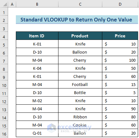
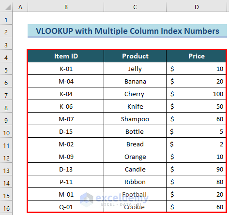
Imagine you’re working in a supermarket, and your worksheet contains information about products, including their Item ID, Product Name, and Price.

1.1 Using Standard VLOOKUP within the Same Worksheet

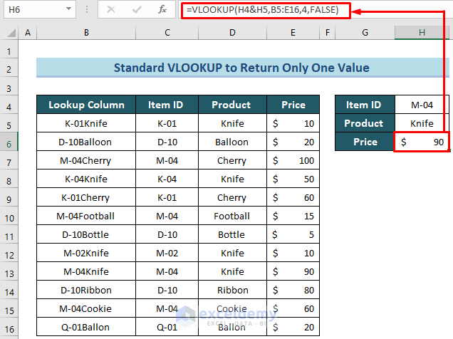
Suppose you want to find the price of a specific product with a particular ID, such as the product Knife with ID M-04. Follow these steps:

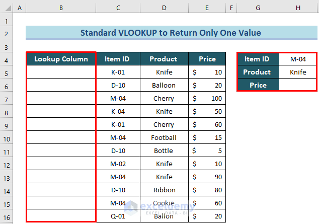
Create a Lookup Column
- Add a new column called Lookup Column to your table array. This column should be the leftmost column because the VLOOKUP function searches from left to right.
- Create a table anywhere in the worksheet where you want to get the price for the product Knife with ID M-04.

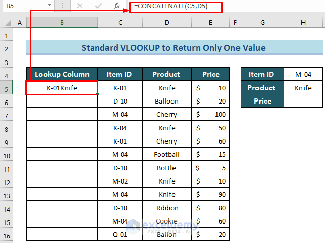
- In this column, use the CONCATENATE function to merge the values from the Item ID and Product columns. For example, if cell C5 contains the Item ID and cell D5 contains the Product, enter the following formula in cell B5:

=CONCATENATE(C5,D5)

- Press Enter to get the merged values.

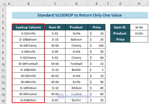
- Use the Fill handle feature to copy the same formula down to B16.

Apply VLOOKUP
- In cell H6 (or any other cell where you want the result), use the VLOOKUP function to find the price for the product Knife with ID M-04. The formula should look like this:

=VLOOKUP(H4&H5,B5:E16,4,FALSE)

Press Enter.

Formula Breakdown

H4 & H5 concatenates the values in the Lookup Column (created earlier) to search for the specific product.
B5:E16 represents the table array containing the data.
4 indicates the column index (in this case, the Price column).
[range_lookup] is set to FALSE for an exact match.

By following these steps, you’ll be able to use VLOOKUP to retrieve a single value from multiple columns within the same worksheet.

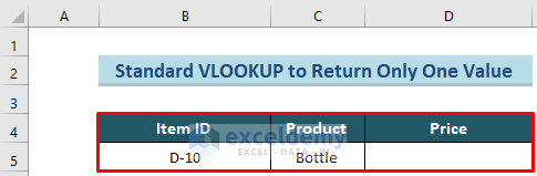
1.2 Using VLOOKUP across Different Worksheets

Suppose your data array is in a different worksheet (let’s call it M01), and you want to perform the same operation in another worksheet (M02). Here’s how:

Set up a table in the M02 worksheet where you want to find the price using the VLOOKUP function.

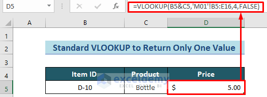
In cell D5 (or any other cell where you want the result), enter the following formula to retrieve the price from the M01 worksheet:

=VLOOKUP(B5&C5,'M01'!B5:E16,4,FALSE)

Press Enter.

Formula Breakdown

B5 & C5 concatenates the values from the Item ID and Product columns.
‘M01’!B5:E16 specifies the table array in the M01 worksheet.
4 represents the column index (the Price column).
[range_lookup] is set to FALSE for an exact match.

By following these steps, you’ll obtain the lookup value from multiple columns in a different worksheet using VLOOKUP.

Method 2 – Using Multiple VLOOKUP Functions

2.1 Using Multiple VLOOKUP functions within the Same Worksheet

Suppose you have two tables in the same worksheet—one with Item ID and Product columns, and the other with Product and Price columns. Your goal is to find the price using a nested VLOOKUP formula. Follow these steps:

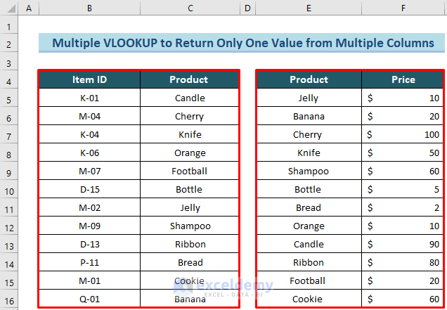
Set up a table anywhere in the worksheet where you want to retrieve the value from multiple columns.

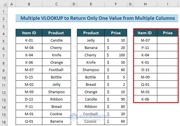
In cell I5 (or any other cell where you want the result), enter the following formula:

=VLOOKUP(VLOOKUP(H5,B$5:C$16,2,FALSE),E$5:F$16,2,FALSE)

Press Enter. This approach allows you to return only one value from multiple columns.

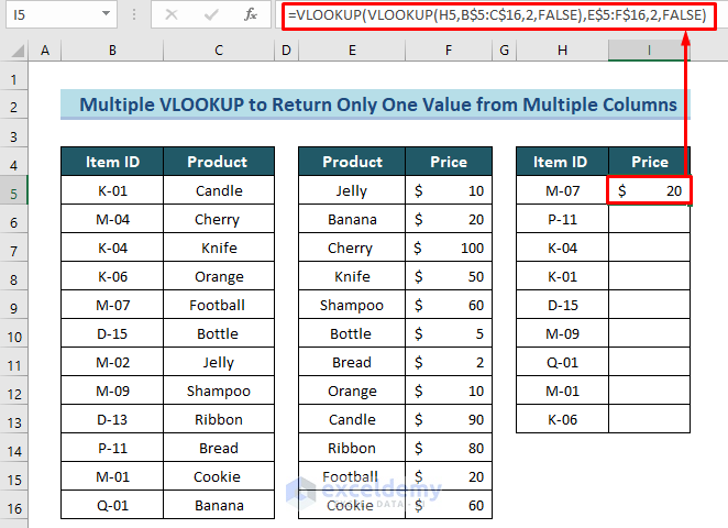
Formula Breakdown

The inner VLOOKUP (VLOOKUP(H5, B$5:C$16, 2, FALSE)) pulls the Product based on the lookup value.
The outer VLOOKUP then searches for the price using the product as the lookup value.
B$5:C$16 represents the first table array (Item ID and Product).
E$5:F$16 represents the second table array (Product and Price).

Use the Fill handle tool to copy down the same formula dynamically.

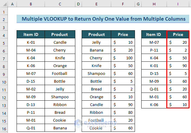
This approach allows you to return only one value from multiple columns.

2.2 Using Multiple VLOOKUP functions across Different Worksheets

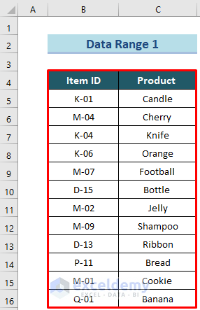
Now let’s consider a scenario where the data tables are in different worksheets (W1 and W2). Follow these steps:

Create Data Tables
- In the W1 worksheet, set up a table called Data Range 1 containing relevant data.

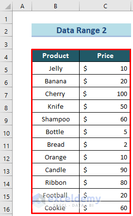
- In the W2 worksheet, create another table called Data Range 2.

Create a Result Table
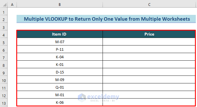
- In a new worksheet, create a table where you want to display the results.

Apply Nested VLOOKUP
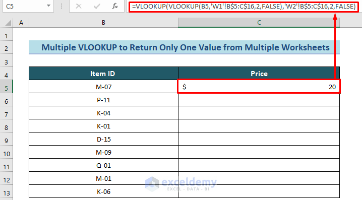
- In cell C5 (or any other cell where you want the result), enter the following formula:

=VLOOKUP(VLOOKUP(B5,'W1'!B$5:C$16,2,FALSE),'W2'!B$5:C$16,2,FALSE)

Press Enter to return only Price from multiple columns lookup.

Formula Breakdown

The inner VLOOKUP (VLOOKUP(B5, ‘W1’!B$5:C$16, 2, FALSE)) retrieves the product from the W1 sheet.
The outer VLOOKUP then searches for the price using the product as the lookup value in the W2 sheet.
‘W1’!B$5:C$16 represents the first table array.
‘W2’!B$5:C$16 represents the second table array.

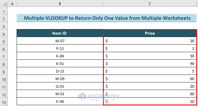
Use the Fill Handle tool to apply the same formula for the rest of the Item IDs.

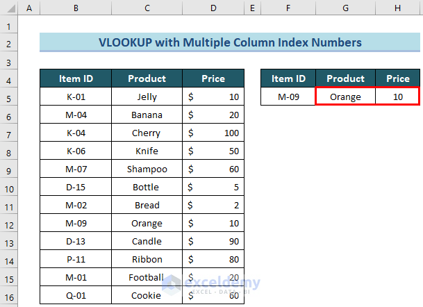
Applying Excel VLOOKUP with Multiple Column Index Numbers

Suppose you need to look up multiple values simultaneously using a single VLOOKUP function. You can achieve this by using multiple-column index numbers. For example, if you have Item ID, Product, and Price in your dataset, and you want to return both the product and price for the item with ID M-09, follow these steps:

Set up a table where you want to display the results.

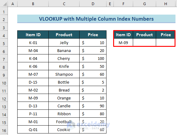
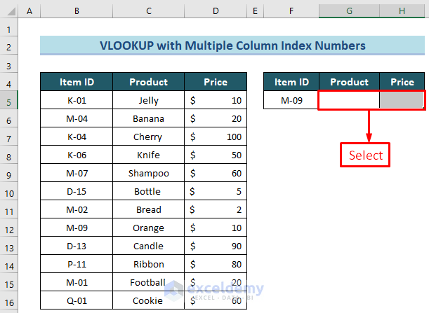
Select cells G5:H5 (or any other range where you want the results).

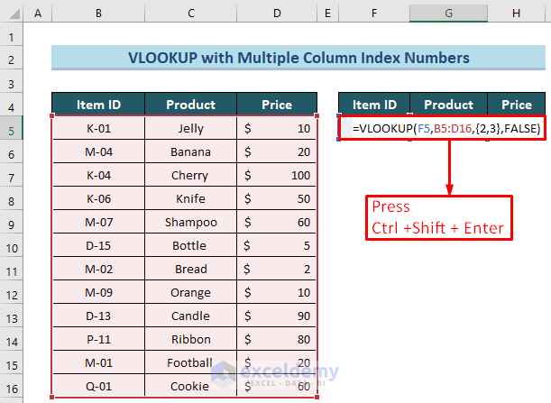
Insert the following formula and press Ctrl+Shift+Enter (or just Enter for Excel 365 users):

=VLOOKUP(F5,B5:D16,{2,3},FALSE)

- This formula returns multiple lookup values with multiple-column index numbers.
- {2, 3} specifies the column indices for Product and Price.