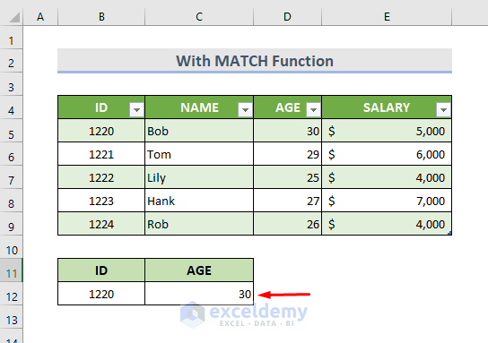
Method 1 – Using a Dynamic VLOOKUP with the MATCH Function
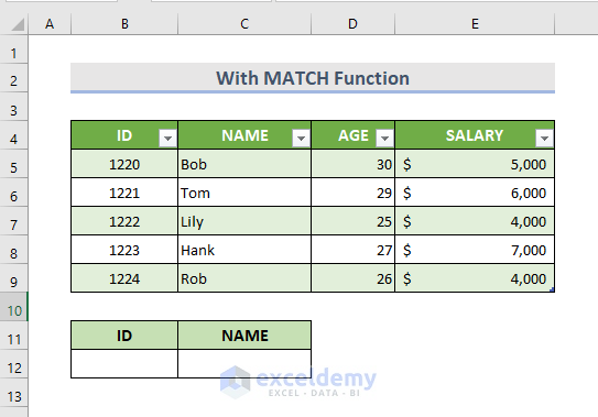
This is the sample dataset.
To find an employee’s information according to the ID and display it in C12:
STEPS:
- Create a drop-down list in C11 using Data Validation.
- Enter the ID in B12 and select C12.
- Enter the following formula:
=VLOOKUP($B12,Table1,MATCH(C$11,Table1[#Headers],0),0)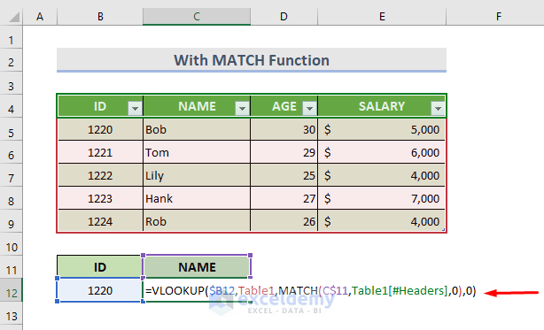
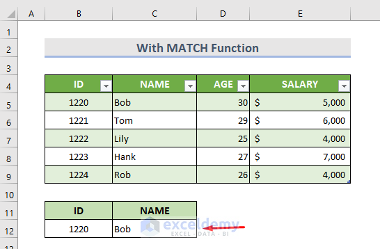
- Press Enter to see the result.
- Change the header name in the drop-down list to see other information.
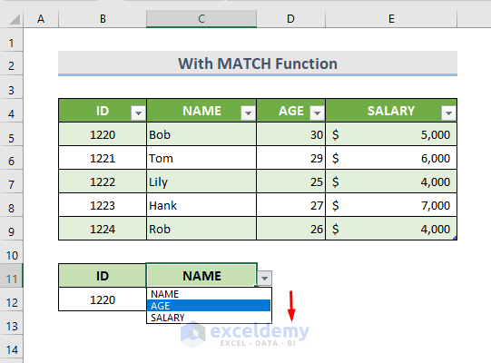
- Select the option and press Enter to see the result.
Formula Breakdown
➤ MATCH(C$11,Table1[#Headers],0)
looks up the exact match of value (C11) in Table 1 Headers. Makes the row number absolute.
➤ VLOOKUP($B12,Table1,MATCH(C$11,Table1[#Headers],0),0)
returns the exact match from the whole dataset in B12 . The column number is absolute.
Read More: 7 Practical Examples of VLOOKUP Function in Excel
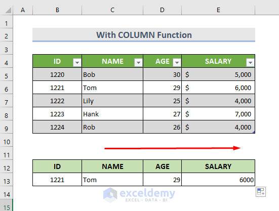
Method 2 – Using the VLOOKUP with a Dynamic Column Reference in Excel
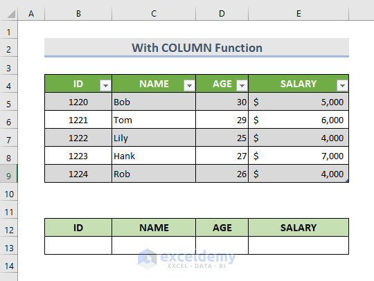
STEPS:
- Enter the lookup ID.
- Select C13.
- Enter the formula:
=VLOOKUP($B$13,Table2,COLUMN(B1),FALSE)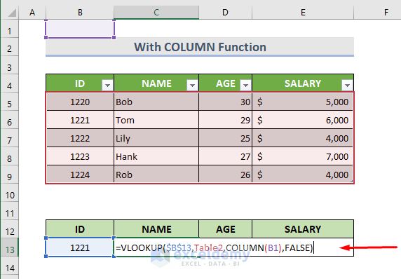
- Press Enter.
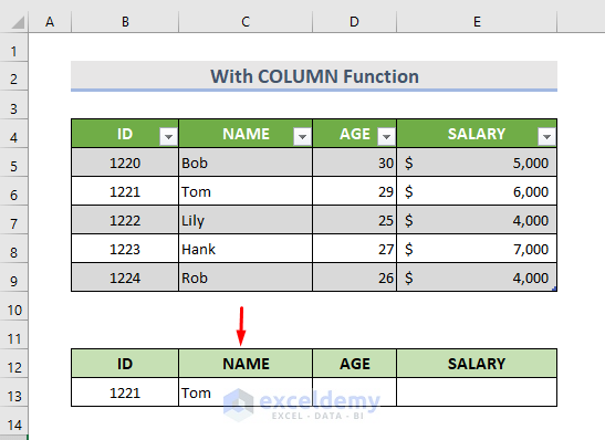
- Drag the Fill Handle icon to the right till E13 and see the result.
Formula Breakdown
➤ COLUMN(B1)
helps to get the column number.
➤ VLOOKUP($B$13,Table2,COLUMN(B1),FALSE)
returns the exact match of B13 from the array (Table 2). Makes the column & row numbers absolute.
Method 3 – Using the VLOOKUP with the Excel COLUMNS Function
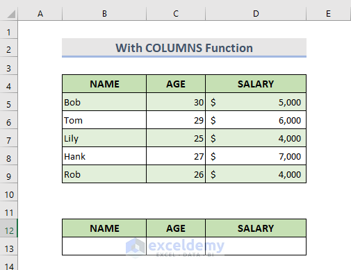
STEPS:
- Enter a name from the list in the Name column of the primary data table in B13 .
- Select C13.
- Enter the formula:
=VLOOKUP($B13,$B$4:$D$9,COLUMNS($B4:C4),0)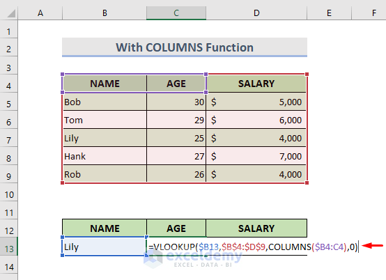
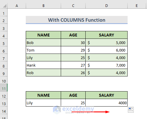
- Press Enter.
- Drag the Fill Handle to the right to see the result.
Formula Breakdown
➤ COLUMNS($B4:C4)
counts the number of columns in B4:C4. Makes the first column absolute.
➤ VLOOKUP($B13,$B$4:$D$9,COLUMNS($B4:C4),0)
returns the exact match in B13 from the array B4:D9. Makes the column and row numbers absolute.
Read More: How to Make VLOOKUP Case Sensitive in Excel
Download Practice Workbook
Download the following workbook and exercise.
Read More: 10 Best Practices with VLOOKUP in Excel
Related Articles
- VLOOKUP Example Between Two Sheets in Excel
- Transfer Data from One Excel Worksheet to Another Automatically with VLOOKUP
- VLOOKUP from Another Sheet in Excel
- How to Use VLOOKUP Formula in Excel with Multiple Sheets
- How to Remove Vlookup Formula in Excel
- How to Apply VLOOKUP to Return Blank Instead of 0 or NA
- How to Hide VLOOKUP Source Data in Excel
- How to Copy VLOOKUP Formula in Excel
<< Go Back to Excel VLOOKUP Function | Excel Functions | Learn Excel
Get FREE Advanced Excel Exercises with Solutions!
