How to Lookup Value from Another Sheet in Excel (3 Easy Methods)

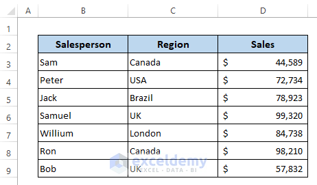
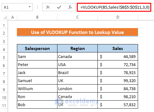
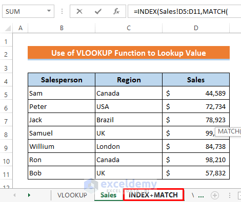
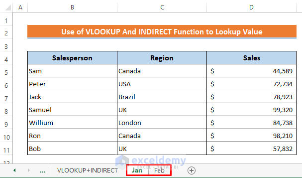
There are a few relatively simple methods you can use to look up data from another sheet in Excel. To demonstrate the capabilities of these methods, let’s use the following dataset, which represents salespersons and their total sales in different regions.

Method 1 – Using the VLOOKUP Function to Lookup Value from Another Sheet in Excel

The VLOOKUP function is one of the most common and simplest ways to fetch information from a lookup table. It finds the desired value in the first column in a range and returns the contents of a specific cell to its right. For this example, we’ll fetch the sales for Jack and Bob.

Steps:

• Write the following formula in Cell C5–

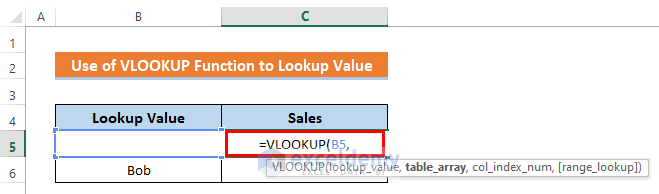
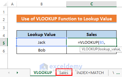
• Click on the sheet where your table array is located. In the example, the sales data is located in the sheet named ‘Sales’.

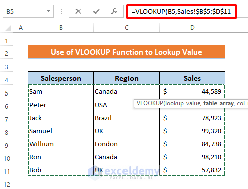
• Drag over the lookup table array (starting with the column where the lookup value is) with your mouse and press F4 to lock the reference so the array doesn’t move if you copy the formula.

• Later, put down the column number in the selected array from that contains the data you want to extract. In this example, the range starts with the name and the sales numbers are in the third column on the right, so the number is “3.”
• For the last argument, type “0” to force Excel to look for an exact match.
• The complete formula will be as follows-

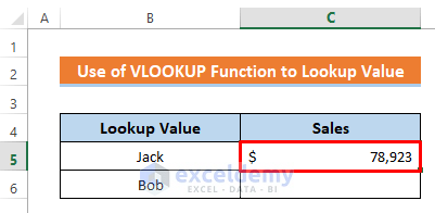
• Finally, just hit Enter.

• You will now have the sales output for Jack.

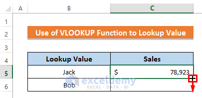
• To find the output for Bob, just drag down the Fill Handle to the next row.

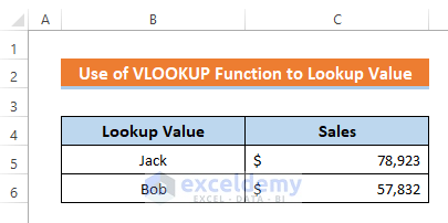
Here’s the final output.

Method 2 – Combining INDEX and MATCH Functions to Lookup Value From Another Sheet

You can also use INDEX and MATCH functions to look up a value from another sheet. The INDEX function is used to return a value or a cell range at a provided location in a table. The MATCH function is used to search for a specified item in a range of cells and then returns the relative position of that item in the range, so it can be used as an argument for the INDEX function. Follow the steps below to find Jack’s sales values from the example.

Steps:

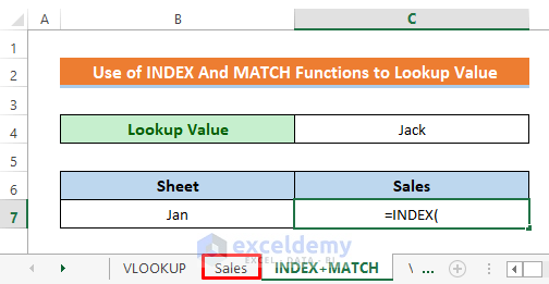
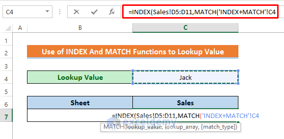
• In Cell C7 type-

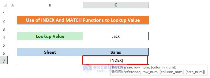
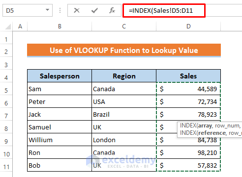
• After that go to the sales sheet by clicking on the sheet title.

• Then select the range D5:D11 from where we’ll extract the output.

• For the next argument, start the MATCH() function, like this:

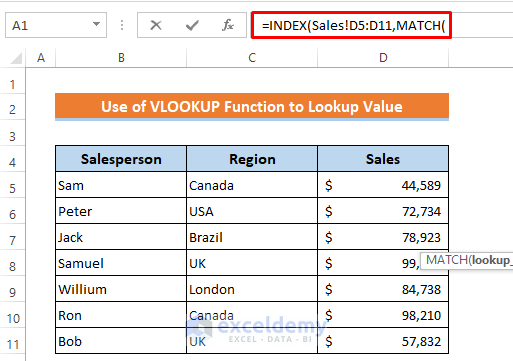
• Return to the sheet where you need to display the result.

• Then select the cell where the lookup value is located.

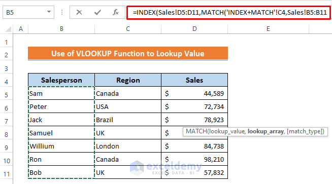
• Go to the ‘Sales’ sheet again and select the column range (B5:B11) that contains the lookup value.

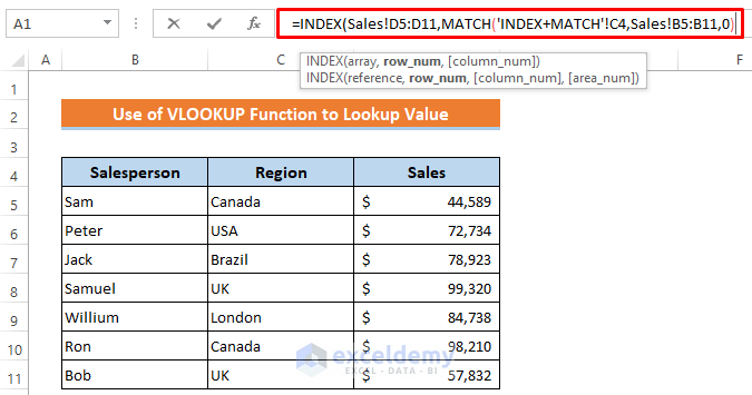
• Lastly, write 0 for the exact match and close all parentheses.
• So, the complete formula will be as follows:

• Finally, just press Enter.

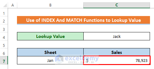
• Then you will get your expected output.

⏬ Formula Breakdown:

➥ MATCH(‘INDEX+MATCH’!C4,Sales!B5:B11,0)
The MATCH function will search for the value ‘Jack’ in the ‘Sales’ sheet between the range B5:B11 and it will return the relative row number-
3

➥ INDEX(Sales!D5:D11,MATCH(‘INDEX+MATCH’!C4,Sales!B5:B11,0))
Finally, the INDEX function will return the value from the range D5:D11 according to the output of the MATCH function and that is-
$78923

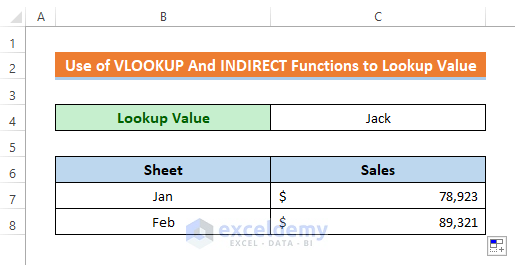
Method 3 – Applying Excel VLOOKUP and INDIRECT Functions to Lookup Value From Another Sheet

You can combine the INDIRECT and VLOOKUP functions to look up a value from different sheets and extract the output from them simultaneously. The INDIRECT function in Excel is used to convert a text string into a valid cell reference.

For this example, we can use two datasets of sales for two consecutive months. Now we’ll find the sales for Jack in both sheets.

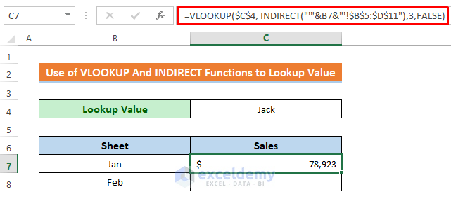
• Write the following formula in Cell C7–

• Later, just press the Enter button for the output.

• Then drag down the Fill Handle icon to get the output from the sheet ‘Feb’.

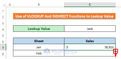
Now we have found the sales for Jack extracted from both sheets.

⏬ Formula Breakdown:

➥ INDIRECT(“‘”&B7&”‘!$B$5:$D$11”)
The INDIRECT function will convert the value of the first argument (B7 = Jan) into a string and concatenate it with “$B$5:$D$11” to return the reference value for a lookup table in a sheet that corresponds to the first argument-
{“Sam”,”Canada”,44589;”Peter”,”USA”,72734;”Jack”,”Brazil”,78923;”Samuel”,”UK”,99320;”Willium”,”London”,84738;”Ron”,”Canada”,98210;”Bob”,”UK”,57832}

➥ VLOOKUP($C$4, INDIRECT(“‘”&B7&”‘!$B$5:$D$11”),3,FALSE)
Finally, the VLOOKUP function will return the value in the third column from the resulting reference range that corrsponds with the value of Cell C4 and that is-
78923

Download Practice Workbook

<< Go Back to Lookup | Formula List | Learn Excel