Dataset Overview
When working with large datasets, you often need to retrieve specific values. Excel provides a powerful feature called lookup tables to help with this task. Let’s explore what lookup tables are and how you can use them effectively.
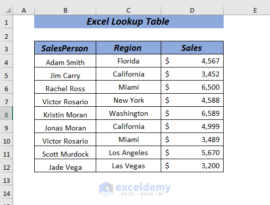
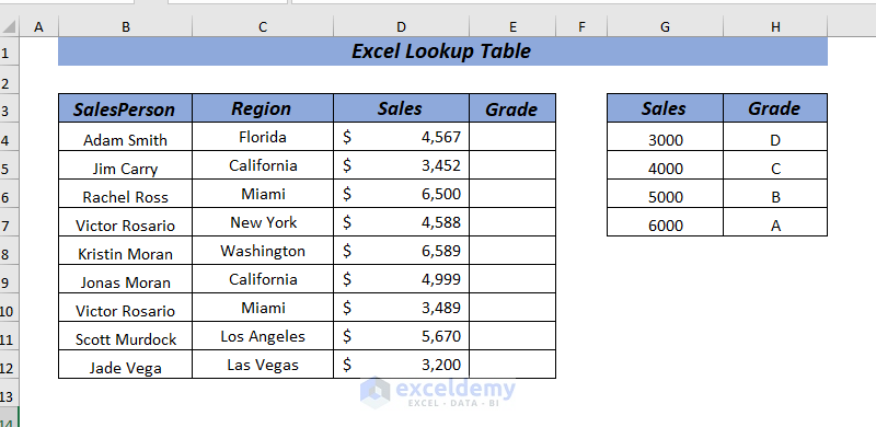
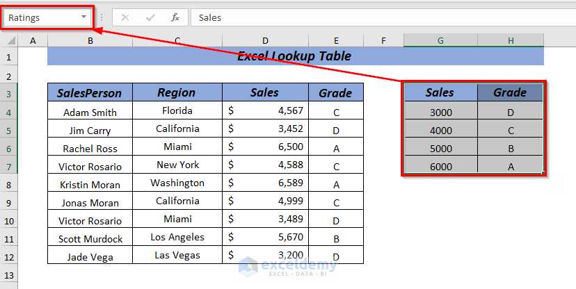
To make the explanation understandable, I’m going to use a dataset of sales information for a particular region. The dataset contains 3 columns. These are SalesPerson, Region, and Sales.
What is Lookup Table?
A lookup table is essentially a reference to a dataset. When you want to fetch data associated with a particular value, you treat the dataset as a lookup table. There are two ways to define a lookup table:
- Using the Total Range of the Dataset:
- You can use the entire range of your dataset as a lookup table.
- This means that any value within the dataset can be looked up using various Excel functions.
- Naming a Specific Range:
- Alternatively, you can name a specific range within your dataset.
- This named range becomes your lookup table.
- You’ll use this name when applying lookup functions like LOOKUP, VLOOKUP, HLOOKUP, XLOOKUP, INDEX, and MATCH.
Advantages of Using Lookup Tables:
- Simplicity: Instead of referring to cell references, you can use descriptive table names for lookups.
- Efficiency: Named tables make your formulas more readable and easier to maintain.
- Flexibility: You can quickly find data associated with specific criteria without complex cell references.
In summary, lookup tables in Excel provide a convenient way to retrieve data from large datasets, making your work more efficient and organized. Remember to choose the approach that best suits your needs—whether it’s using the entire dataset or naming a specific range.
Method 1 – Using Excel LOOKUP Array to Lookup a Table
In Excel, you can utilize the LOOKUP function to perform table lookups. There are two approaches, depending on your dataset and requirements. Let’s explore the array form of using the LOOKUP function.
- Array Form:
- When you have a table (or similar data structure) in Excel, the array form of LOOKUP is useful.
- An array represents a collection of values arranged in rows and columns that you want to search.
- The LOOKUP function scans the first row or column of the array for the specified value and returns a corresponding value from the same position in the last row or column of the array.
To get started:
- Select any cell where you want the result to appear. For example, let’s choose cell G4.
- In cell G4, enter the following formula:
=LOOKUP(F4,B4:D12)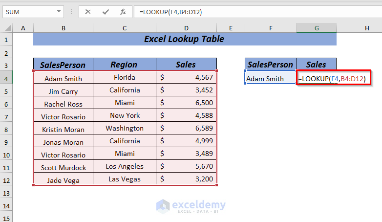
-
- Here:
- F4 is the lookup value (the value you want to find).
- B4:D12 represents the range (array) where you want to search for the lookup value.
- Here:
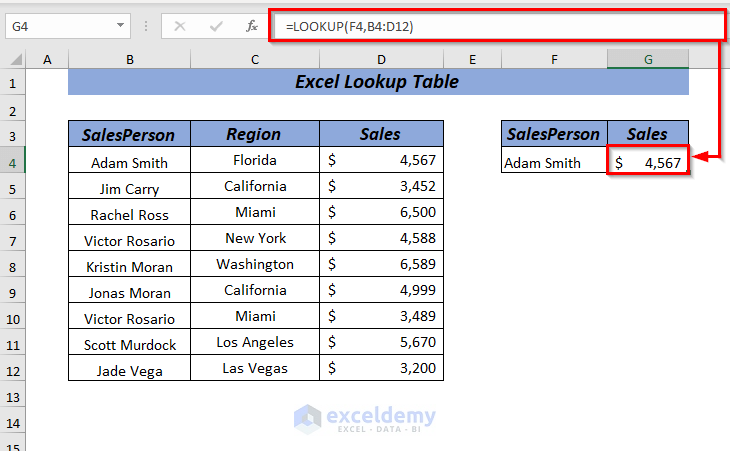
- Press ENTER.
The LOOKUP function will locate the corresponding value associated with the lookup value (Adam Smith) and return it from the same position in the last row or column of the array.
Remember:
- Use the array form of LOOKUP when the values you want to match are in the first row or column of the array.
- Arrange the values in ascending order within the array for accurate results.
Press ENTER, and you’ll retrieve the sales information for the lookup value Adam Smith.
Method 2 – Using Vector Form of LOOKUP to Search a Table
In this method, we’ll use the vector form of the LOOKUP function to search a table in Excel. The vector form allows you to search either a row or a column for a specific value. If you want to specify the range containing the values you want to match, you can use the vector form.
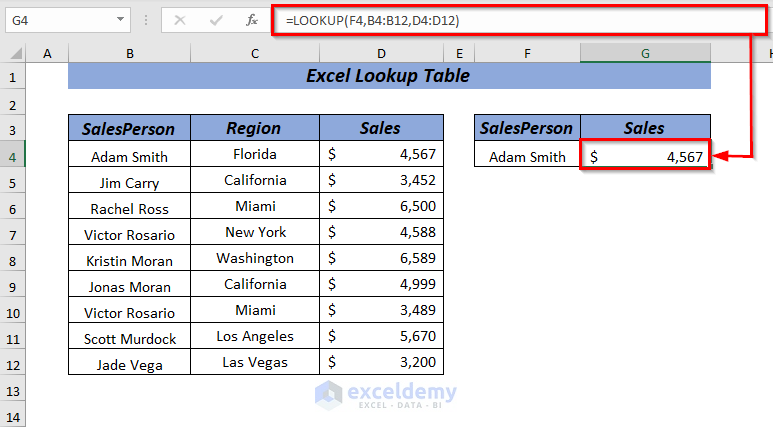
- Select any cell where you want the result to appear. For example, let’s choose cell G4.
- In cell G4, enter the following formula:
=LOOKUP(F4,B4:B12,D4:D12)

-
- Here’s what each part of the formula means:
-
-
- F4 is the lookup value (in this case, the name “Adam Smith”).
- B4:B12 is the lookup vector (the range containing the names).
- D4:D12 is the result vector (the range containing the corresponding sales information).
-
- Press ENTER, and Excel will find the sales information for the lookup value Adam Smith.
Method 3 – Lookup Using an External Table or Range
If you need to look up values from another table or dataset, you can use an external lookup table. Let’s demonstrate this procedure using the dataset provided below. We want to find the corresponding grade based on the sales value, where the grade ranges are predefined.
- Select any cell where you want the result to appear. For example, let’s choose cell E4.
- In cell E4, enter the following formula:
=LOOKUP(D4,$G$3:$H$7)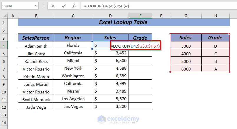
-
- Here’s what each part of the formula means:
- D4 is the lookup value (the sales value).
- $G$3:$H$7 is the lookup vector (the external table containing sales ranges and corresponding grades). We use absolute references to reuse the formula for other cells.
- Here’s what each part of the formula means:
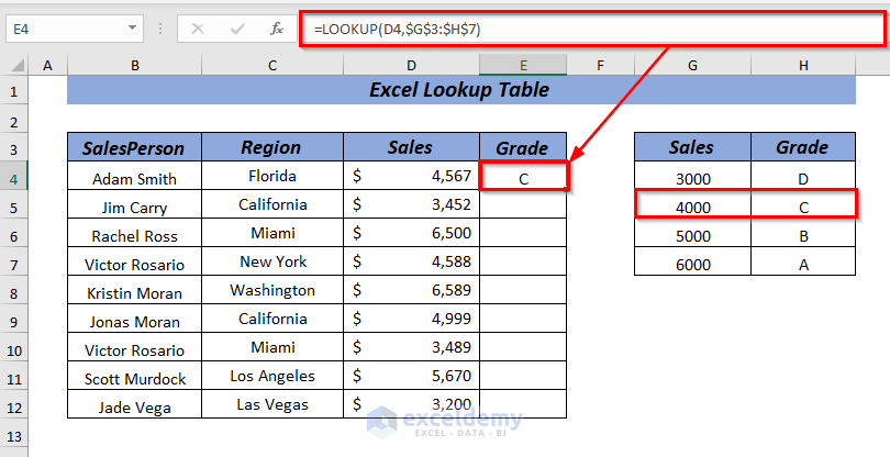
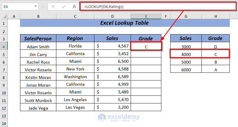
- Press ENTER, and Excel will find the corresponding grade based on the sales value.
-
- Here’s a breakdown of what happened:
- Lookup Value: The value we were searching for was $4567.
- Lookup Table: The lookup table contained sales values and their corresponding grades.
- Nearest Value: LOOKUP started searching from the value $4567 and continued until it found a value that was less than or equal to $4567. In this case, it found $5000 (which is greater than $4567 but the closest value in the table).
- Assigned Grade: Since $5000 corresponds to Grade C in the lookup table, LOOKUP returned Grade C for the value $4567.
- Here’s a breakdown of what happened:
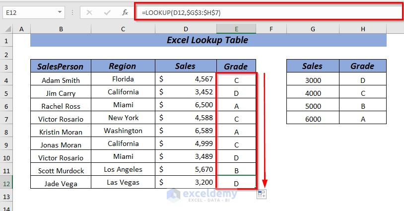
Use the Fill Handle to AutoFill the formula for the remaining cells. The Fill Handle is a convenient way to copy formulas down a column or across a row.
- Click on the cell containing the LOOKUP formula (E4 in our example).
- Hover over the small square at the bottom-right corner of the cell (this is the Fill Handle).
- Click and drag the Fill Handle down to fill the formula into the cells below (E5, E6, and so on).
Excel will automatically adjust the lookup values and return the corresponding grades for each sales value.
Remember to double-check the results to ensure they make sense based on your lookup table.
Method 4 – Lookup Using Named Range in Excel
- Select the range of cells that you want to use as your lookup table. In this case, we’ve already named it Ratings.
- To name the range, go to the Formulas tab, click on Name Manager, and then click New.
- Enter the name Ratings and specify the range (e.g., A1:A10).
- Find the corresponding grade based on the sales value in cell D4.
- In cell E4, enter the following formula:
=LOOKUP(D4,Ratings) 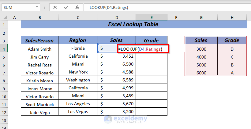
-
- Here:
- D4 is the lookup value (sales value).
- Ratings is the named range (lookup table).
- Grade represents the corresponding grade you want to retrieve.
- Here:
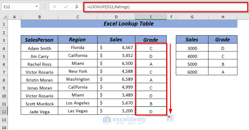
- Press ENTER:
- Excel will search for the exact or closest value of D4 in the Ratings range and return the corresponding grade.
- To apply the same formula to other cells, use the Fill Handle:
- Click and drag the small square at the bottom-right corner of cell E4 down to fill the formula for the rest of the cells.
Method 5 – Using VLOOKUP to Look Up Data in a Table
The VLOOKUP function in Excel allows you to retrieve values from a lookup table. It’s particularly useful when you want to search for data in a table organized vertically.
Here are the steps:
- Select any cell where you want the result to appear. For example, let’s say you’ve chosen cell G4.
- In cell G4, enter the following formula:
=VLOOKUP(F4,B4:D12,3,FALSE)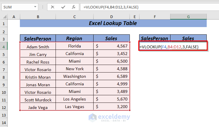
-
- Here:
- F4 is the lookup value (the value you want to find in the table).
- B4:D12 represents the table array (the range of cells containing your data).
- 3 specifies the column index number (in this case, the third column contains the desired information).
- FALSE ensures an exact match (use TRUE for an approximate match).
- Here:
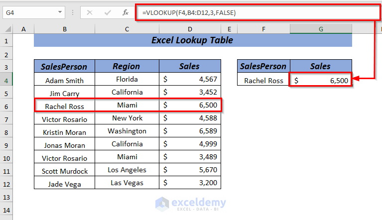
- After typing the formula, press the ENTER key. Excel will return the sales information for the SalesPerson named Rachel Ross based on the lookup value in cell F4.
Method 6 – Using HLOOKUP to Look Up Data in a Table
The HLOOKUP function is useful when you want to find values located in a row across the top of a lookup table. It allows you to look down a specified number of rows to retrieve data. Let’s go through the process step by step:
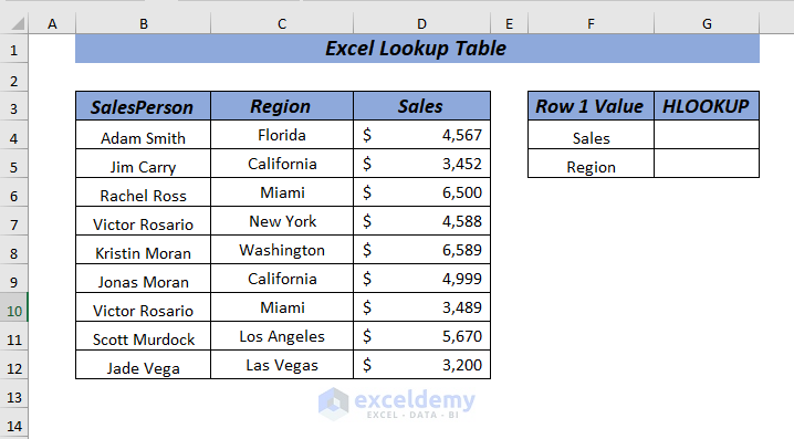
Scenario 1 – Retrieving Sales Information
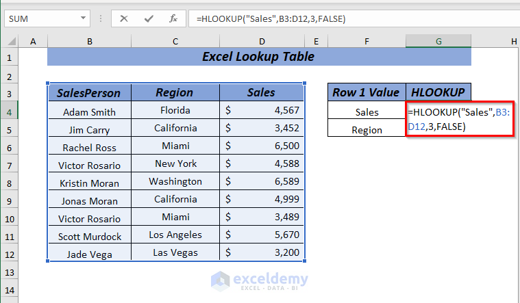
- Select any cell where you want the result to appear. For example, let’s say you’ve chosen cell G4.
- In cell G4, enter the following formula:
=HLOOKUP("Sales",B3:D12,3,FALSE)-
- Here:
-
-
- “Sales” is the lookup value (the column header you’re searching for).
- B4:D12 represents the table array (the range of cells containing your data).
- 3 specifies the row index number (in this case, the third row contains the desired information).
- FALSE ensures an exact match.
-
- After typing the formula, press the ENTER key. Excel will return the sales information for the third row.
You also can use the following formula both will give you the same result.
=HLOOKUP(F4,B3:D12,3,FALSE)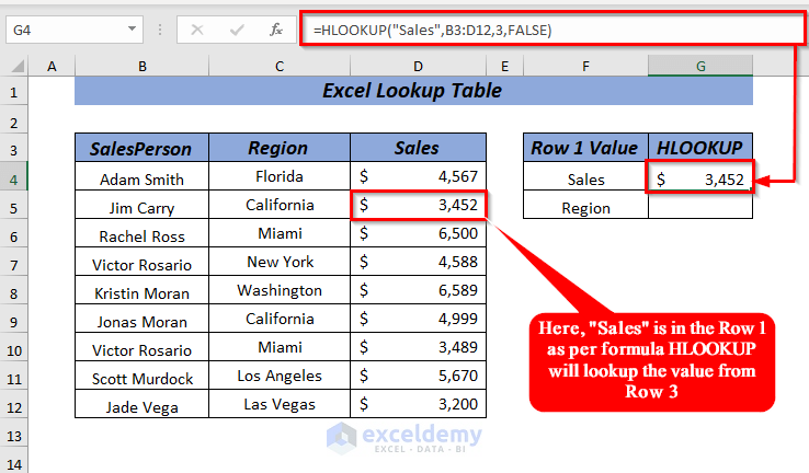
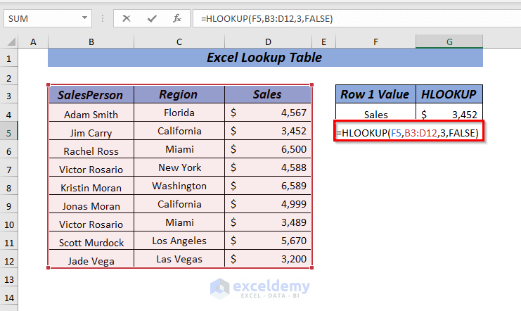
Scenario 2 – Retrieving Region Information
- Select cell G5.
- In cell G5, enter the following formula:
=HLOOKUP(F5,B3:D12,3,FALSE)-
- Here:
- F5 is the lookup value (you can also use cell references).
- B4:D12 is the table array.
- 3 specifies the row index number (again, the third row).
- Here:
- Press Enter. Excel will return the region information for the third row (according to the dataset).
You also can use the following formula both will give you the same result.
=HLOOKUP(“Region”,B3:D12,3,FALSE)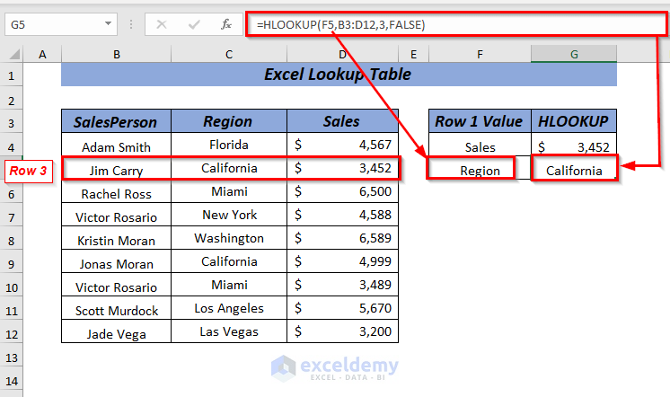
Method 7 – Using XLOOKUP to Look Up Data in a Table
The XLOOKUP function is an improved version of the traditional lookup functions in Excel. It works bidirectionally, meaning you can search for values both horizontally and vertically. Note that XLOOKUP is available in Microsoft 365.
Here’s how you can use XLOOKUP:
- Select any cell where you want the result to appear. For example, let’s say you’ve chosen cell G4.
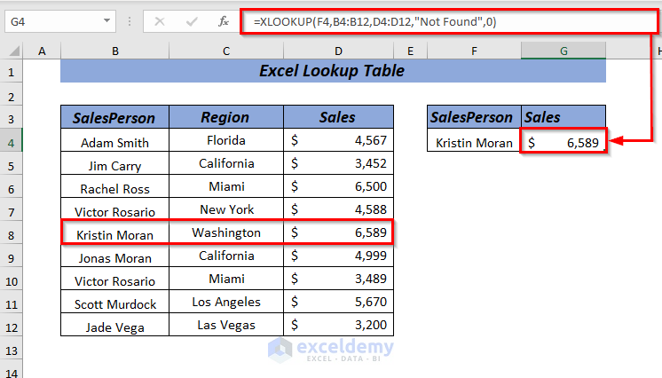
- In cell G4, enter the following formula:
=XLOOKUP(F4,B4:B12,D4:D12,"Not Found",0)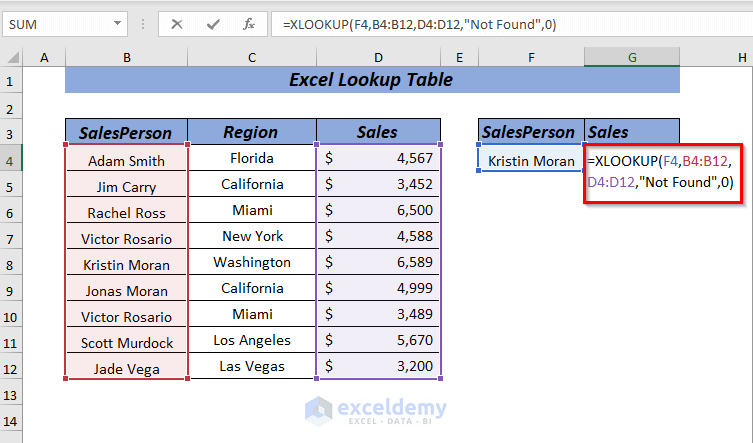
-
- Here:
- F4 is the lookup value (the value you want to find in the table).
- B4:B12 represents the lookup array (the range of cells containing your data).
- D4:D12 is the return array (the corresponding values you want to retrieve).
- “Not Found” specifies what to display if no match exists.
- 0 ensures an exact match (use 1 for approximate match).
- Here:
- After typing the formula, press the ENTER key. Excel will return the associated result for the lookup value from the return array. For example, if you’re looking for sales information related to the SalesPerson Kristin Moran, this formula will provide the relevant data.
Method 8 – Using INDEX-MATCH Formula to Look Up Data in a Table
The combination of INDEX function and MATCH function is a powerful way to retrieve data from a table. It allows you to search for a value and return a corresponding value from another column. Here’s how you can use it:
- Select any cell where you want the result to appear. For example, let’s say you’ve chosen cell G4.
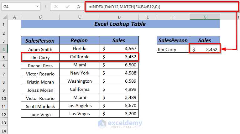
- In cell G4, enter the following formula:
=INDEX(D4:D12,MATCH(F4,B4:B12,0))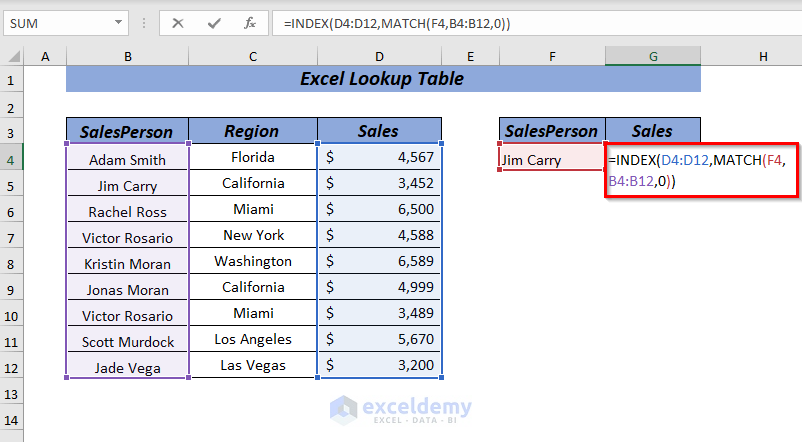
-
- Here:
- D4:D12 represents the array of values you want to retrieve (in this case, sales data).
- MATCH(F4, B4:B12, 0) finds the position of the lookup value (SalesPerson name) in the lookup array (B4:B12). The 0 ensures an exact match.
- Here:
- After typing the formula, press the ENTER key. Excel will return the sales information for the SalesPerson Jim Carry.
Things to Remember
- Always ensure that the values in your lookup array (B4:B12) are sorted in ascending order. Otherwise, you may encounter a #N/A error.
- The lookup value (SalesPerson name) should match exactly with the values in the main table in Excel.
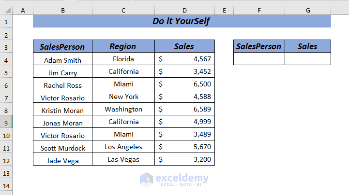
Practice Section
Feel free to practice using the provided workbook.
Download to Practice
You can download the practice workbook from here:
<< Go Back to Lookup | Formula List | Learn Excel
Get FREE Advanced Excel Exercises with Solutions!

This was very helpful thank you, but there is one step that i am needing to know how to do. ill use your example. you have your column here for lookups. you have two vicotr rosario rows. one for miami and one for new york. if i wanted to pull just victor for miami, what syntax would i use?
Hi Kevin!
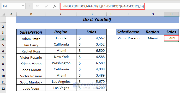
It brings me great joy to know that you found our blog helpful. You are most welcome. As for your query, you can use the following formula:
=INDEX(D4:D12,MATCH(1,(F4=B4:B12)*(G4=C4:C12),0))To be more clear about the cell references look at the image below:
Regards,
Nafis
ExcelDemy