Lookup and Return Multiple Values Concatenated into One Cell in Excel

In Microsoft Excel, there are a number of suitable techniques to lookup a criterion and then return multiple values concatenated into one cell based on that criterion. In this article, you’ll learn all available methods to extract corresponding values concatenated into a single cell with proper illustrations.

How to Lookup and Return Multiple Values Concatenated into One Cell: 4 Methods

1. Use of TEXTJOIN Function to Lookup and Extract Multiple Values Joined into Single Cell

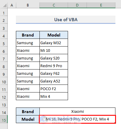
In the following dataset, there are a number of smartphone models with their brands. We’ll extract the model names of a specified brand and then concatenate them into a single cell. By using the TEXTJOIN function, we can meet the requirement easily as this function concatenates a list or range of texts using a delimiter.

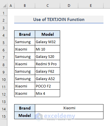
For example, we want to concatenate all model names of Xiaomi smartphones into one cell. So, the required formula in the output cell C15 will be:

After pressing Enter, you’ll be shown all the model names of Xiaomi in a cell at once.

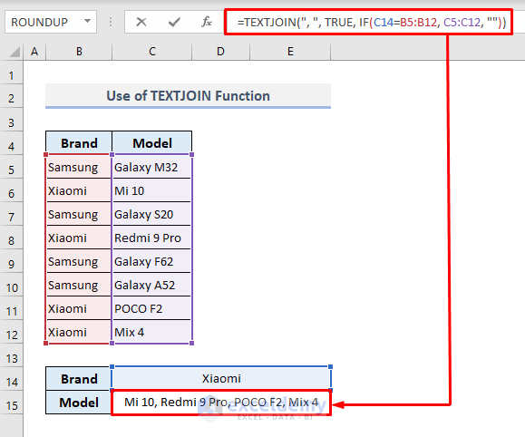
2. Use of VBA to Lookup and Return Multiple Values Concatenated into One Cell

We can also create a user-defined function with the VBA and then concatenate multiple cells into one cell based on the specified conditions.

📌 Step 1

➤ Press ALT+F11 to open the VBA window.

➤ Select the Module option from the Insert tab.

➤ In the new module window, copy and paste the following codes:

Option Explicit

Function CONCATIF(LookupRange As Range, LookupVal As Variant, _

ConcatRange As Range, Optional Separator As String = ",") As Variant

Dim i As Integer

Dim Result As String

On Error Resume Next

If LookupRange.Count <> ConcatRange.Count Then

    CONCATIF = CVErr(xlErrRef)

    Exit Function

End If

For i = 1 To LookupRange.Count

    If LookupRange.Cells(i).Value = LookupVal Then

        Result = Result & Separator & ConcatRange.Cells(i).Value

    End If

Next i

If Result <> "" Then

    Result = VBA.Mid(Result, VBA.Len(Separator) + 1)

End If

CONCATIF = Result

Exit Function

End Function

Sub Lookup_and_Concat()

End Sub

➤ Press F5 to run the codes.

➤ Return to the Excel spreadsheet by pressing ALT+F11 again.

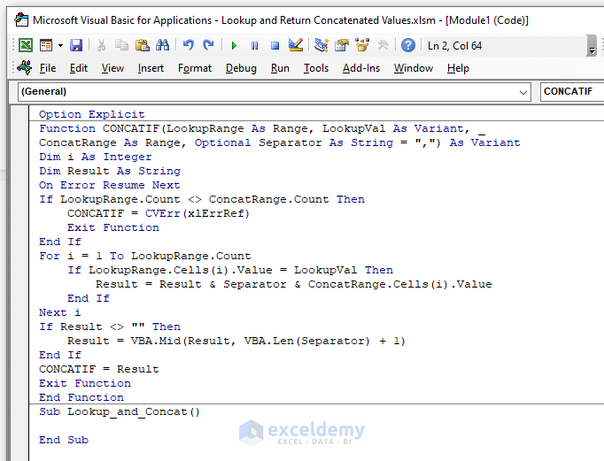
So, we’ve just created a user-defined function and that is:

=CONCATIF(LookupRange, LookupVal, ConcatRange, [Separator])

📌 Step 2

➤ Now select the output cell C15 and type:

➤ Press Enter and you’re done.

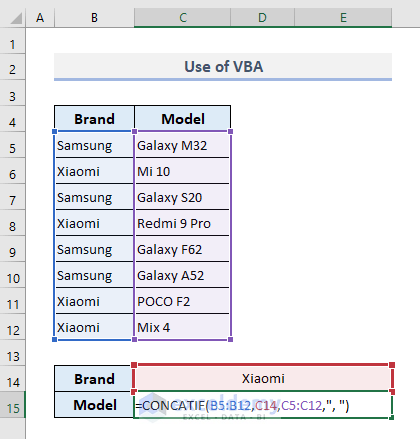
You’ll find the concatenated values in a single cell as shown in the screenshot below.

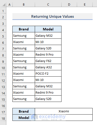
3. Lookup and Return Multiple Unique Values Concatenated into One Cell

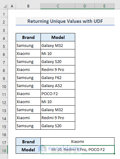
Now let’s consider another scenario where the smartphone model names can be present with duplicates in Column C. Such cases are common with worksheets that have a large amount of data. What we’ll do here is extract and concatenate all smartphone models of a specified brand into a single cell but display each model name only once if duplicates are found.

In the output cell C18 the required formula under the specified criteria will be:

After pressing Enter, you’ll find all the smartphone model names of the Xiaomi brand concatenated into a single cell but without any duplication.

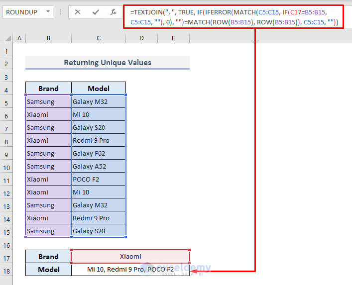
🔎 How Does the Formula Work?

• IFERROR(MATCH(C5:C15, IF(C17=B5:B15, C5:C15, “”), 0), “”): This part of the formula checks if the defined condition in cell C17 matches with the values in the range of cells B5:B15 and returns the corresponding row numbers of the values. If duplication is found for a value then the row number returns for the first value. Thus this part of the formula returns the following array:

{“”;2;””;4;””;””;7;2;””;4;””}

• IF(IFERROR(MATCH(C5:C15, IF(C17=B5:B15, C5:C15, “”), 0), “”)=MATCH(ROW(B5:B15), ROW(B5:B15)), C5:C15, “”): This part is the third argument (text1) of the TEXTJOIN function which defines the statements to be concatenated. Here the values from Column C will be extracted based on the row numbers found in the previous step. So, the return array here will be:

{“”;”Mi 10″;””;”Redmi 9 Pro”;””;””;”POCO F2″;””;””;””;””}

• Finally, the entire formula will concatenate the values obtained in the preceding step with the defined delimiter- Comma (,).

4. Use of VBA to Lookup and Return Multiple Unique Values Concatenated into One Cell

We can also use the VBA codes to formulate another user-defined function that will be applied to concatenate multiple unique values into a single cell.

📌 Step 1

➤ Press ALT+F11 and open the VBA window.

➤ Activate a new module from the Insert tab and then paste the following codes in the new module window:

Option Explicit

Function CONCATUNIQUE(LookupValue As String, LookupTable As Range, Col_Num As Integer)

Dim i As Long

Dim j As Integer

Dim Result As String

For i = 1 To LookupTable.Columns(1).Cells.Count

  If LookupTable.Cells(i, 1) = LookupValue Then

    For j = 1 To i - 1

    If LookupTable.Cells(j, 1) = LookupValue Then

      If LookupTable.Cells(j, Col_Num) = LookupTable.Cells(i, Col_Num) Then

        GoTo Skip

      End If

    End If

    Next j

    Result = Result & " " & LookupTable.Cells(i, Col_Num) & ","

Skip:

  End If

Next i

CONCATUNIQUE = Left(Result, Len(Result) - 1)

End Function

Sub Concatenate_Unique()

End Sub

➤ Press F5 and you’re done.

The user-defined function we’ve just created is:

=CONCATUNIQUE(LookupValue, LookupTable, Col_Num)

📌 Step 2

➤ Return to your Excel spreadsheet by pressing ALT+F11 once again.

➤ In the output cell C18, type:

➤ Press Enter.

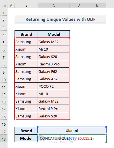
You’ll get the return values in a single cell as shown in the picture below.

Download Practice Workbook

You can download the Excel workbook that we’ve used to prepare this article.

Concluding Words

I hope all these methods mentioned above will now help you to apply them in your Excel spreadsheet to lookup and return multiple values concatenated into a single cell. If you have any questions or feedback, please let me know in the comment section. Or you can check out our other articles related to Excel functions on this website.

<< Go Back to Lookup | Formula List | Learn Excel