This is an overview. 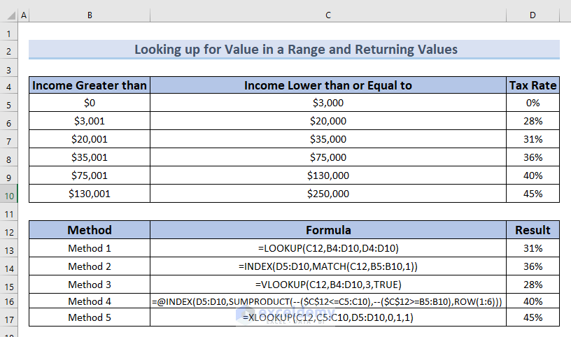
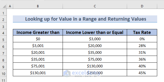
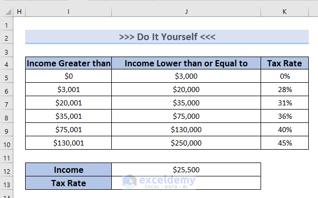
The following dataset has the Income Greater than, Income Lower than or Equal, and Tax Rate columns.
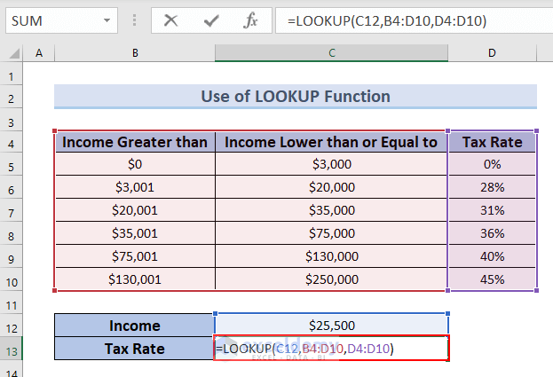
Method 1 – Using the LOOKUP Function to Find and Return a Value in a Range
Steps:
- Enter the following formula in C13.
=LOOKUP(C12,B4:D10,D4:D10)
Formula Breakdown
- C12 is the lookup value, (Income).
- B4:D10 is the entire dataset.
- D4:D10 is the range (Different Tax Rate) from which the match value for the lookup value will be returned.
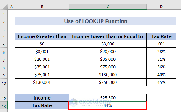
- LOOKUP(C12,B4:D10,D4:D10) → becomes
- Output: 31%
You can see the result in C13.
Method 2 – Combining the INDEX and MATCH Functions to Lookup and Return a Value in a Range
Steps:
- Enter the following formula in C13.
=INDEX(D5:D10,MATCH(C12,B5:B10,1))
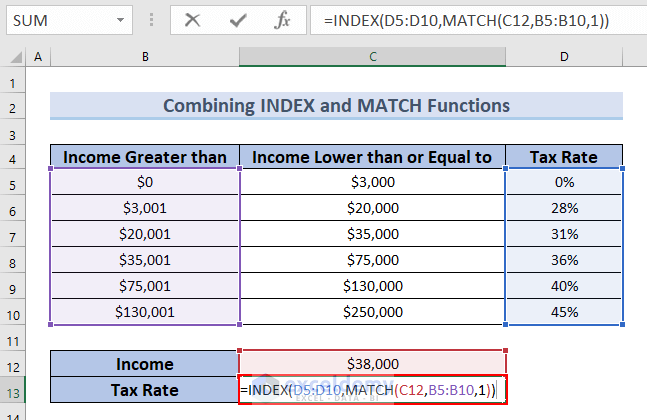
Formula Breakdown
- C12 is the lookup value (Income).
- D5:D10 is the range (Different Tax Rate) from which the match value for the lookup value will be returned.
- B5:B10 is the range for the lookup value (Lower limit of Income for a particular Tax Rate).
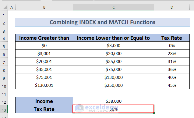
- INDEX(D5:D10,MATCH(C12,B5:B10,1)) → it becomes
- Output: 36%
- Press ENTER.
You can see the result in C13.
Method 3 – Using the VLOOKUP Function
Steps:
Enter the following formula in C13.
=VLOOKUP(C12,B4:D10,3,TRUE)
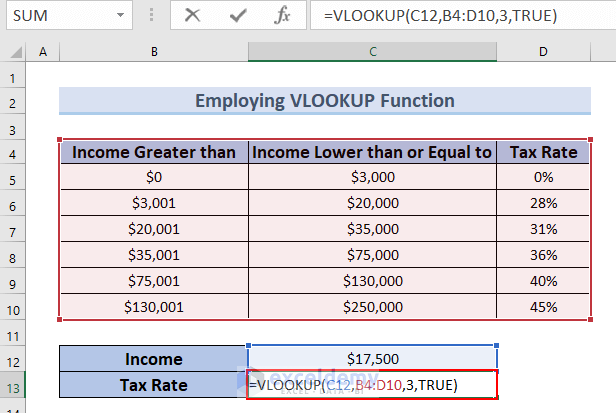
Formula Breakdown
- C12 is the lookup value, (Income).
- B4:D10 is the entire dataset.
- 3 indicates that the value will be returned from the third column(Tax rate).
- TRUE indicates that Excel will return a value if the lookup value exists in any data range.
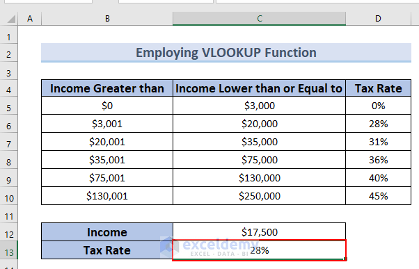
- VLOOKUP(C12,B4:D10,3,TRUE) → it becomes
- Output: 28%
- Press ENTER.
You can see the result in C13.
Method 4 – Combining the INDEX, SUMPRODUCT, and ROW Functions to Search and Extract a Value
Steps:
- Enter the following formula in C13.
=@INDEX(D5:D10,SUMPRODUCT(--($C$12<=C5:C10),--($C$12>=B5:B10),ROW(1:6)))
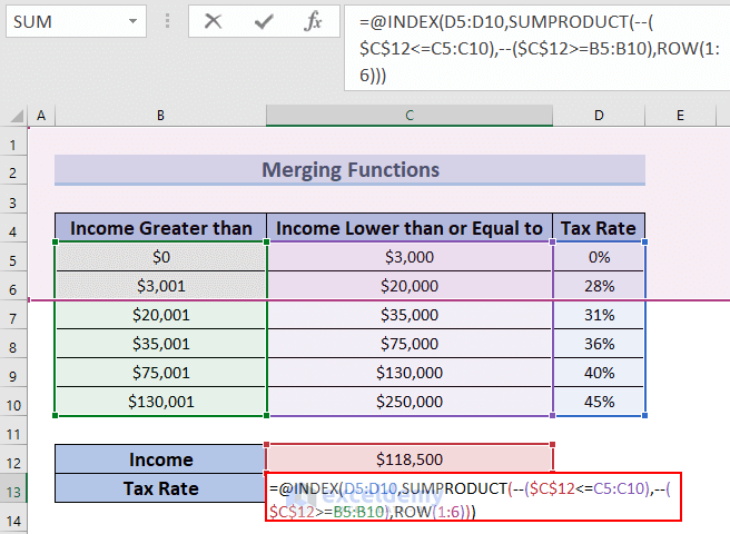
Formula Breakdown
- C12 is the lookup value, (Income).
- D5:D10 is the range (Different Tax Rate) from which the match value for the lookup value will be returned.
- B5:B10 is the upper limit of different ranges (Income lower than or Equal to)
- C5:C10 is the lower limit of different ranges (Income Greater than).
- 1:6 refers to the first six rows.
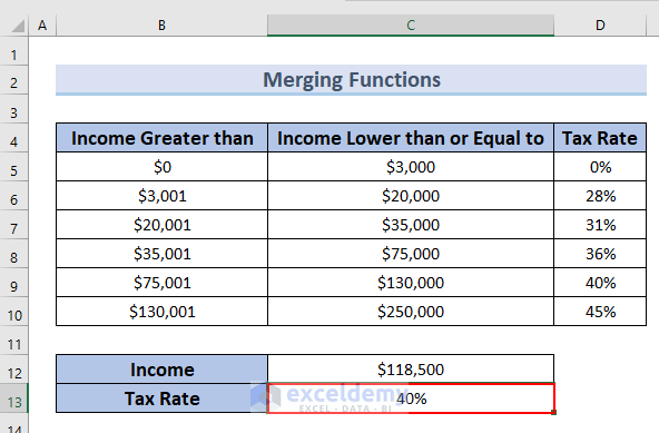
- @INDEX(D5:D10,SUMPRODUCT(–($C$12<=C5:C10),–($C$12>=B5:B10),ROW(1:6))) → it becomes
- Output: 40%
Note: You have to select the exact number of rows in your dataset.
- Press ENTER.
You can see the result in C13.
Method 5 – Using the XLOOKUP Function to Return a Value
Steps:
- Enter the following formula in C13.
=XLOOKUP(C12,C5:C10,D5:D10,0,1,1)
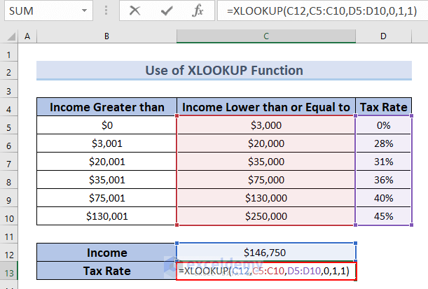
Formula Breakdown
- C12 is the lookup value (Income).
- C5:C10 is the range for the lookup value (Upper limit of Income for a particular tax rate).
- D5:D10 is the range (Different Tax Rate) from which the match value for the lookup value will be returned.
- 0 indicates that no value will be shown if the lookup value isn’t found.
- The first 1 in the argument indicates that if an exact match is not found, then the formula will return the next smaller value.
- The second 1 indicates that the search will be started in the beginning of your dataset.
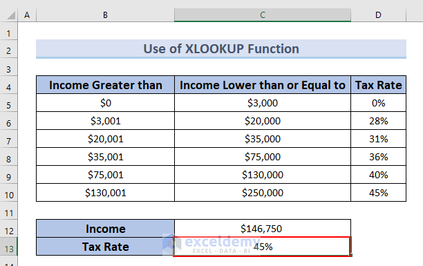
- XLOOKUP(C12,C5:C10,D5:D10,0,1,1) → it becomes
- Output: 45%
- Press ENTER.
You can see the result in C13.
Practice Section
Practice here.
Download Practice Workbook
Download the Excel file and practice.
<< Go Back to Lookup | Formula List | Learn Excel
Get FREE Advanced Excel Exercises with Solutions!
