Here’s an overview of the article, which represents a simplified application of the LOOKUP function in Excel. You’ll learn more about the dataset as well as the methods and functions under different criteria in the following sections of this article.
Introduction to the LOOKUP Function
⏺ Function Objective
The LOOKUP function looks up a value in the one-row or one-column range.
⏺ Available in
Excel for Office 365, Excel 2019, Excel 2016, Excel 2013, Excel 2011 for Mac, Excel 2010, Excel 2007, Excel 2003, Excel XP, Excel 2000.
⏺ Syntax
The LOOKUP function is available in 2 formats: the Vector form and the Array form.
Syntax in Vector Form:
⏺ Arguments Explanations (Vector Form)
| Argument | Required/Optional | Explanations |
|---|---|---|
| lookup_value | Required | A value that LOOKUP explores in the first vector. Lookup_value can be a number, text, a logical value, or a name or reference that refers to a value. |
| lookup_vector | Required | A range that includes only one row or one column. The values in lookup_vector can be text, numbers, or logical values. |
| [result_vector] | Optional | A range that incorporates only one row or column. The result_vector statement must be the same size as lookup_vector. It has to be the exact size. |
Important Note to Remember: The values in lookup_vector must be put in ascending order: …, -2, -1, 0, 1, 2, …, A-Z, FALSE, TRUE; otherwise, LOOKUP might not return the accurate value. Uppercase and lowercase text are identical.
[/wpsm_box]
Syntax in Array Form:
⏺ Arguments Explanations (Array Form)
| Argument | Required/Optional | Explanations |
|---|---|---|
| lookup_value | Required | A value that LOOKUP explores in the first vector. Lookup_value can be a number, text, a logical value, or a name or reference that refers to a value. |
| array | Required | A range of cells that contains text, numbers, or logical values that you want to compare with lookup_value. |
⏺ Return Parameter (Vector and Array Forms)
In both formats, the LOOKUP function returns the output for the look-up value.
How to Use the LOOKUP Function in Excel: 2 Easy Ways
Method 1 – Vector Form of the LOOKUP Function in Excel
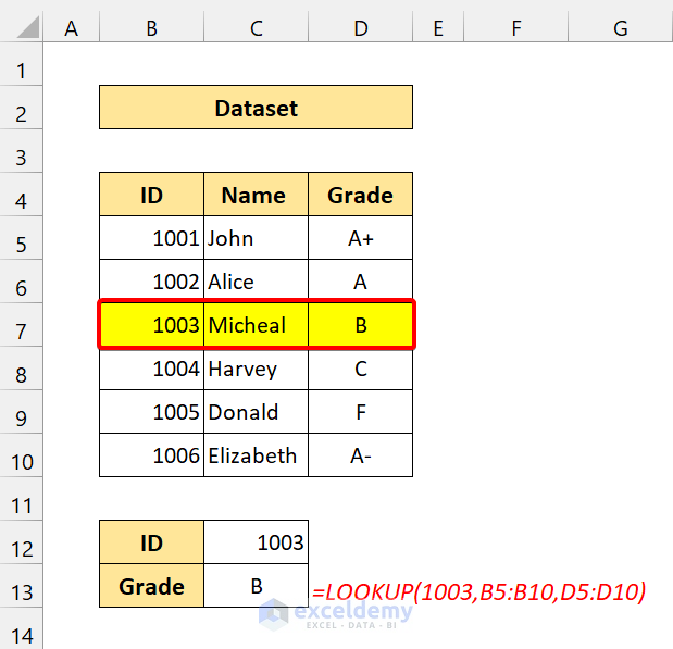
The vector form of the LOOKUP function will explore one row or one column of data for a particular value, then fetch the data from the exact position in another row or column.
You can see this from this example. Our lookup value was 1003. The LOOKUP function first searched for this value. Then, it returns the corresponding result from the same row.
Read More: How to Use LOOKUP Function Among Multiple Sheets in Excel
Method 2 – Array Form of the LOOKUP Function in Excel
The array format of LOOKUP peeks in the first row or column of an array for the particular value and returns a value from the same place in the last row or column of the array. We must use this form of LOOKUP when the values that we want to match are in the first row or column of the array.
When we use the array form of the LOOKUP function, the LOOKUP function acts based on the array dimensions. Your array looks taller which means it has more rows than columns. The LOOKUP will behave like the VLOOKUP function in that case.
If your array is wider, it will work like the HLOOKUP function. Wider means it has more columns than rows.
Formula for Vertical Array:
=LOOKUP(E5,B5:C9)
The formula for Horizontal Array:
=LOOKUP(E6,C11:G12)
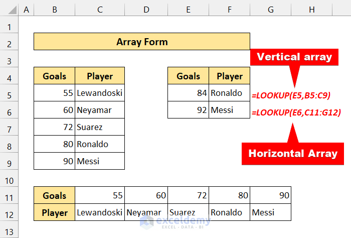
We have the same dataset. We placed the array differently. The first one is the vertical format, and the second one is the horizontal format.
How to Use the LOOKUP Function in Excel: 5 Suitable Examples
Example 1 – Find the Last Non-empty Cell in Column
Take a look at the following dataset:
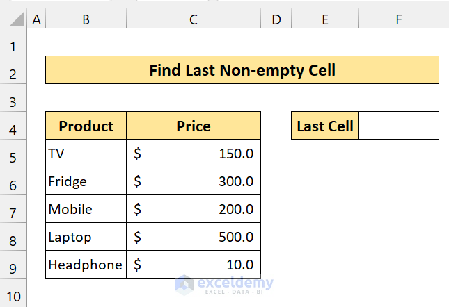
- Use the following formula in Cell F4:
=LOOKUP(2,1/(B:B<>""),B:B)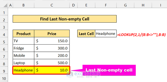
Example 2 – Find the Last Non-Empty Cell in Row
- Enter the following formula in cell F4 and press Enter.
=LOOKUP(2,1/(5:5<>""),5:5)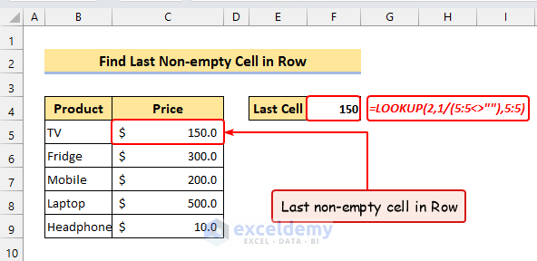
You will get the last non-empty cell from the 5th row in cell F4 as shown in the following image.
Example 3 – Find the Latest Value in Excel
This is a dataset of Ballon d’Or from the year 2009 to 2020. Our goal is to find the latest value for Ronaldo.
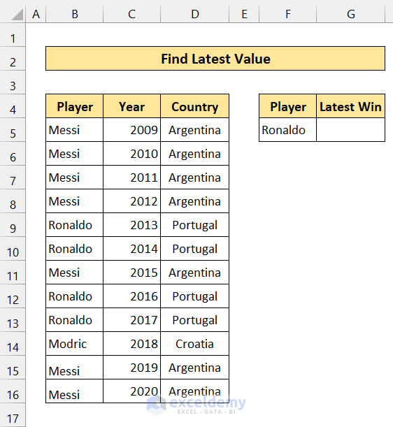
- Use the following formula in Cell G5:
=LOOKUP(2,1/(B5:B16=F5),C5:C16)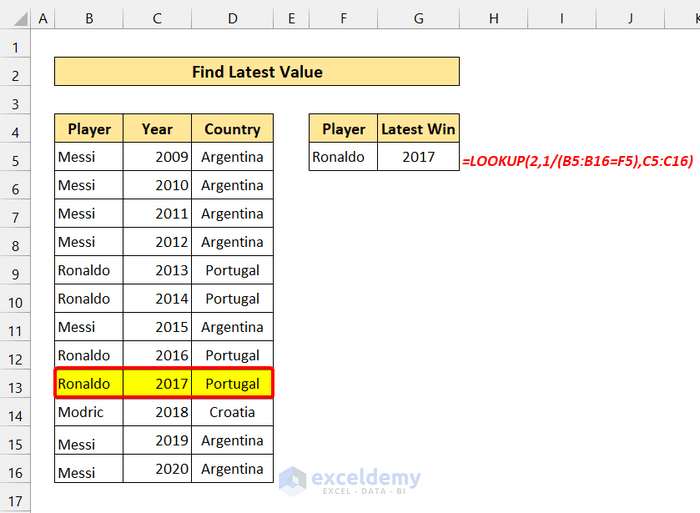
This finds the latest value using the LOOKUP function in Excel.
Example 4 – Find the Grades Based on Marks
We will find a value based on data that is not present in the dataset. But our LOOKUP function array form will find the nearest small value. We can use this to see grades. We have some marks and grades. On the right-hand side, we have a mark that is not in the dataset. Our goal is to find the grade based on that mark.
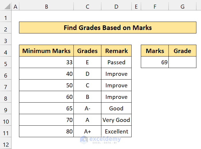
- Use the following formula in Cell G5:
=LOOKUP(F5,B5:C11)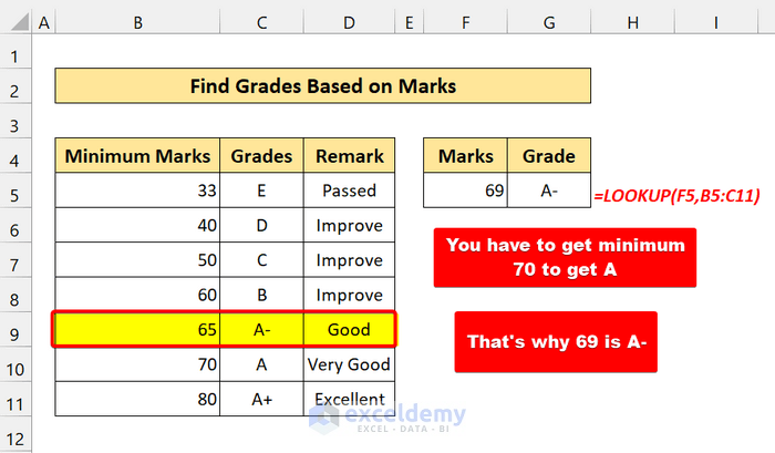
The grade is A- because you have to get 70 to get the grade A. That’s why it chooses the nearest small value A-.
Example 5 – Combine the LOOKUP Function with IF to Show a Message If the Lookup Value Is Empty
We have some codes for products and their prices. We’ll find the price based on the Code.
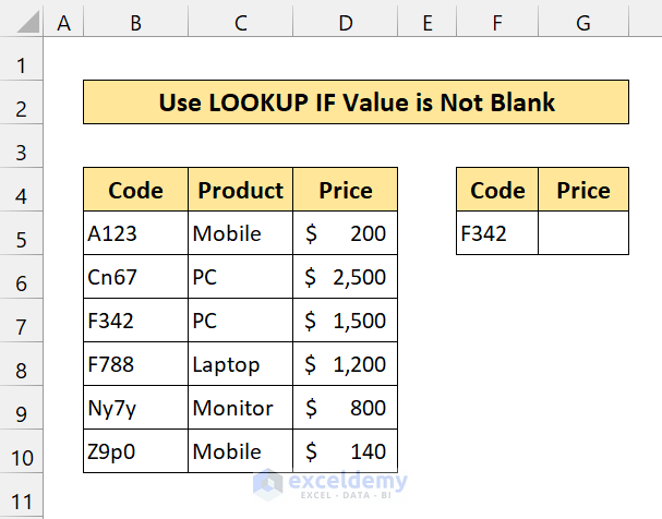
- Enter the following formula in Cell G5:
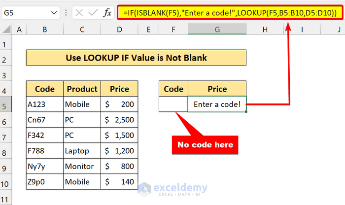
=IF(ISBLANK(F5),"Enter a code!",LOOKUP(F5,B5:B10,D5:D10))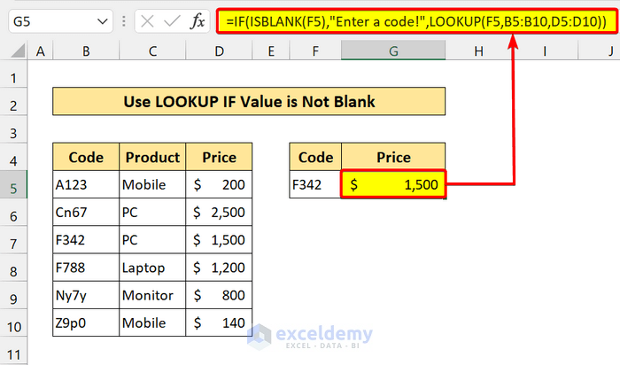
We have successfully found the price based on the code using the LOOKUP function.
- Delete the code.
Excel will tell you to enter a code.
Things to Remember
- Your lookup array must be in ascending order.
- If an array is square or is taller than it is wide (more rows than columns), LOOKUP searches in the first column.
- If the value of lookup_value is less than the smallest value in the first row or column (relying on the array dimensions), LOOKUP returns the #N/A error value.
- When your lookup_value is greater than all values in the range, the LOOKUP function matches the last value.
- The result_vector must be the same size as lookup_vector.
Download the Practice Workbook
<< Go Back to Excel Functions | Learn Excel
Get FREE Advanced Excel Exercises with Solutions!
