While working in Excel, we often need to find a specific value from a dataset. If the dataset is quite large, then it becomes a pretty challenging task to find a value from a huge dataset. So, to solve this problem, we can use the Lookup function of Excel VBA. In this article, we will demonstrate 6 simple, and practical examples to use the VBA Lookup function in Excel. So, let’s start this article and explore these examples.
Excel VBA Lookup Function (Quick View)
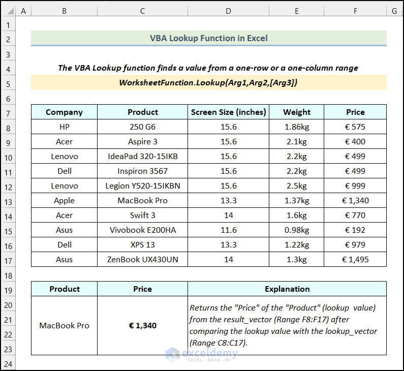
The overview of the VBA Lookup function is demonstrated in the following image. We will discover more about using the VBA Lookup function in different examples in later portions of this article.
Introduction to VBA Lookup Function in Excel
Now, let’s familiarize ourselves with Syntax, Argument, and Return Value subsections of the VBA Lookup function to understand the basics of the function.
Summary:
- The VBA Lookup function finds a value from a one-row or a one-column range.
Syntax:
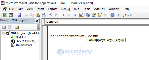
The syntax of the VBA Lookup function is:
WorksheetFunction.Lookup(Arg1,Arg2,[Arg3])Arguments:
| Argument | Required/Optional | Explanation |
|---|---|---|
| Arg1 | Required | The first argument is the lookup value. It can be any text, number, logical values, etc. It can also be a cell reference that refers to a value. |
| Arg2 | Required | This is the range where we will search for our lookup value. This range is also known as the lookup vector. |
| [Arg3] | Optional | This is the range that contains our desired output. It is also known as the result vector. |
Return Value:
The VBA Lookup function returns the value from the result vector after comparing the lookup value with the lookup vector.
Remarks:
- For the VBA Lookup function to work properly, the lookup vector column should be sorted in ascending order first.
- The size of the result vector should be the same as the lookup vector.
How to Use VBA Lookup Function in Excel: 6 Suitable Examples
In this section of the article, we will discuss 6 practical examples of using the VBA Lookup function in Excel. Let’s say, we have the Laptop Prices in Micro Center Store as our dataset. Using this dataset, we will demonstrate the application of the VBA Lookup function in the following sections.

Not to mention, we used the Microsoft Excel 365 version for this article; however, you can use any version according to your preference.
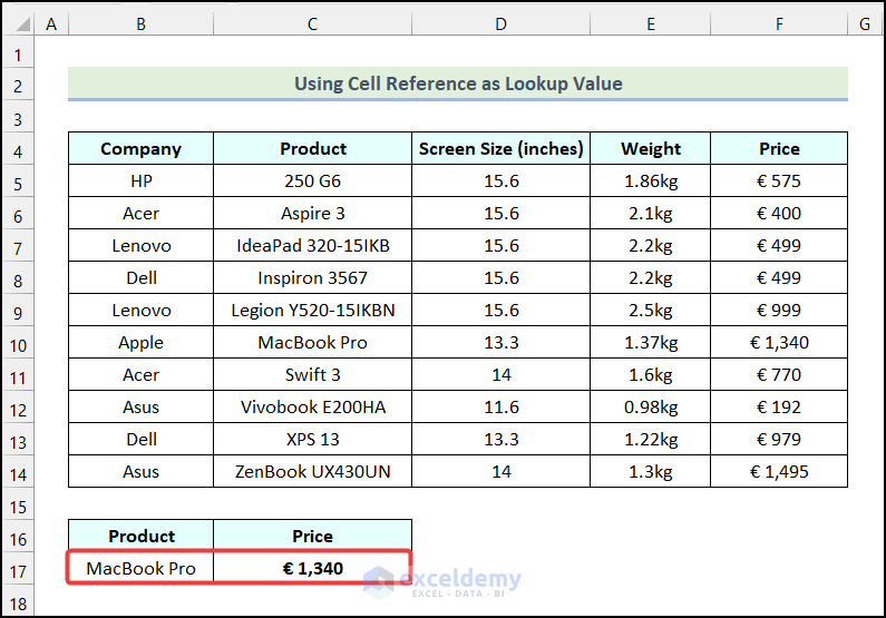
1. Using Cell Reference as Lookup Value
In the first example, we will use the Cell Reference as a lookup value in the VBA Lookup function in Excel. Now let’s follow the steps mentioned below to this.
Step 01: Sort Lookup Vector in Ascending Order
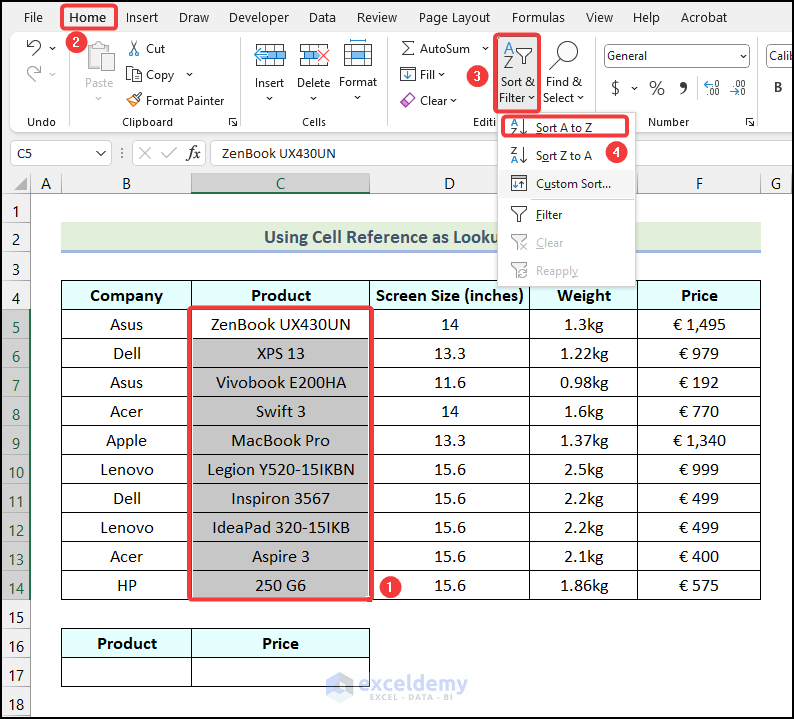
First, you need to Sort the lookup vector in ascending order. Here, we will use the name of the Product as our lookup value. Therefore, our lookup vector will be in the range C5:C14.
- Now, select the cells of the range C5:C14 as shown in the following image.
- After that, go to the Home tab from Ribbon.
- Then, click on the Sort & Filter option from the Editing group.
- Subsequently, choose the Sort A to Z option from the drop-down.
As a result, the Product column will be sorted in ascending order.

Step 02: Insert New Module in VBA Editor
- Firstly, go to the Developer tab from Ribbon.
- After that, choose the Visual Basic option from the Code group.
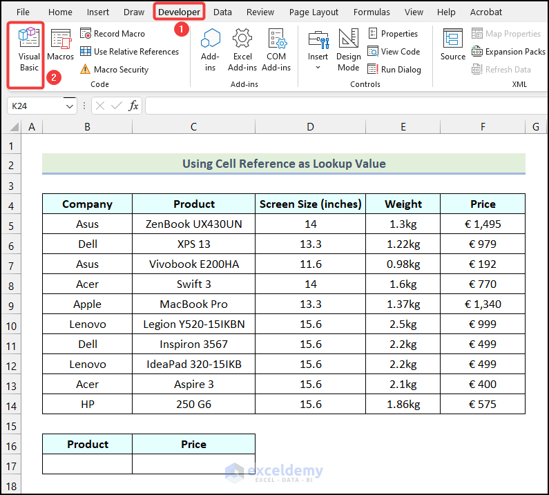
As a result, the Microsoft Visual Basic for Applications window will appear on your worksheet.

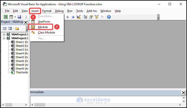
- Now, go to the Insert tab in the Microsoft Visual Basic for Applications window.
- Then, choose the Module option from the drop-down.
Step 03: Write and Save VBA Code in New Module
- Firstly, write the following code in the newly created Module.
Sub lookup_with_cell_reference()
Range("C17").Value = WorksheetFunction.Lookup(Range("B17").Value, _
Range("C5:C14"), Range("F5:F14"))
End Sub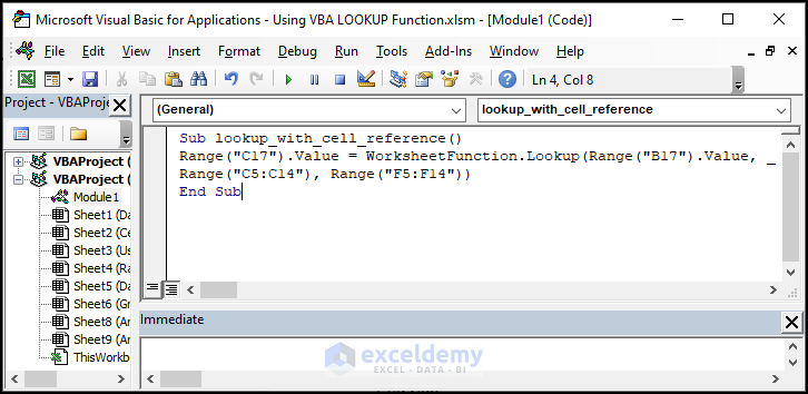
Code Breakdown
- Firstly, we created a sub-procedure named lookup_with_cell_reference.
- After that, we used WorksheetFunction.Lookup Method to find the Price for the lookup value in cell B17 and assign the value to cell C17.
- Then, we ended the sub-procedure.
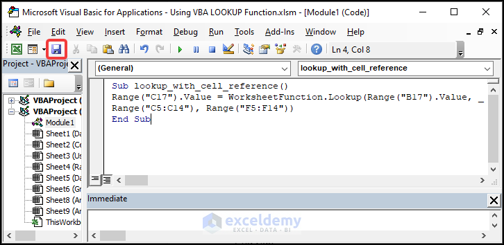
- After writing the code, click on the Save icon.
Step 04: Run Macro to Use VBA Lookup Function
- Firstly, use the keyboard shortcut ALT + F11 to return to the worksheet.
- Now, enter the name of the product in cell B17. This is our lookup value.
- Afterward, use the keyboard shortcut ALT + F8 to open the Macro dialogue box.
- Now, in the Macro dialogue box, choose the lookup_with_cell_reference option.
- Finally, click on Run.
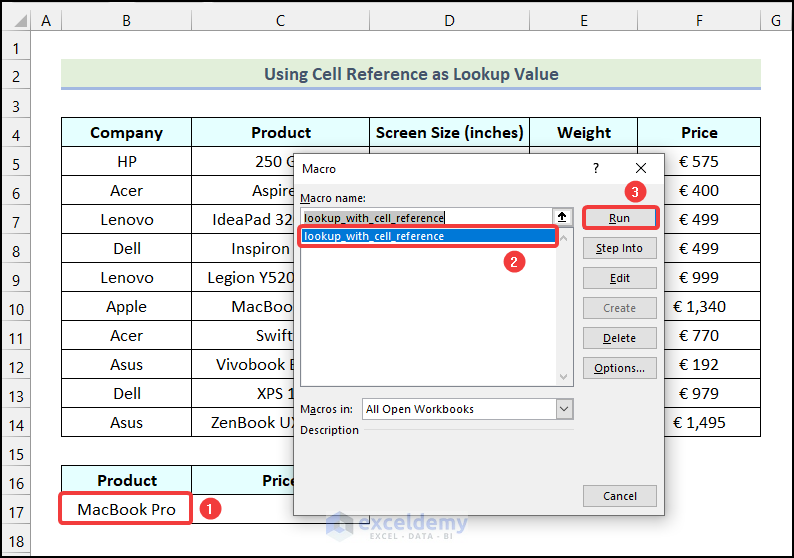
Consequently, the Price of the MacBook Pro will appear in cell C18, as demonstrated in the image below.
2. Utilizing User Input as Lookup Value
In the second example, we will use the user input as our lookup value to find the Price of a laptop using the VBA Lookup function in Excel. We will take the lookup value from the user by utilizing the VBA InputBox function of Excel VBA. Now let’s follow the steps mentioned below to do this.
Steps:
- Firstly, follow the steps mentioned in Step 01 and Step 02 of the first method.
- After that, write the following code in the newly created Module.
Sub user_defined_lookup()
Product = InputBox("Enter the Name of the Product: ")
Range("B17").Value = WorksheetFunction.Lookup(Product, _
Range("C5:C14"), Range("F5:F14"))
End Sub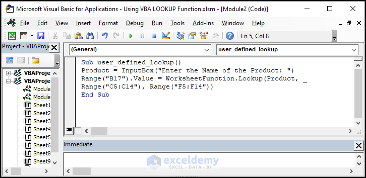
Code Breakdown
- Firstly, we created a sub-procedure named user_defined_lookup.
- Then, introduced a variable named Product.
- After that, we used the InputBox function of Excel to take input from the user and then we assigned the user input into the variable named Product.
- Following that, we used WorksheetFunction.Lookup Method to find the Price for the lookup value defined by the user and assign the value to cell B17.
- Finally, we ended the sub-procedure.
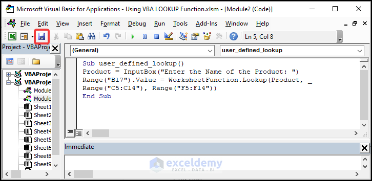
- Then, click on the Save option.
- After that, use the keyboard shortcut ALT + F11 to return to the worksheet.
- Then, enter the name of the product in cell B17. This is our lookup value.
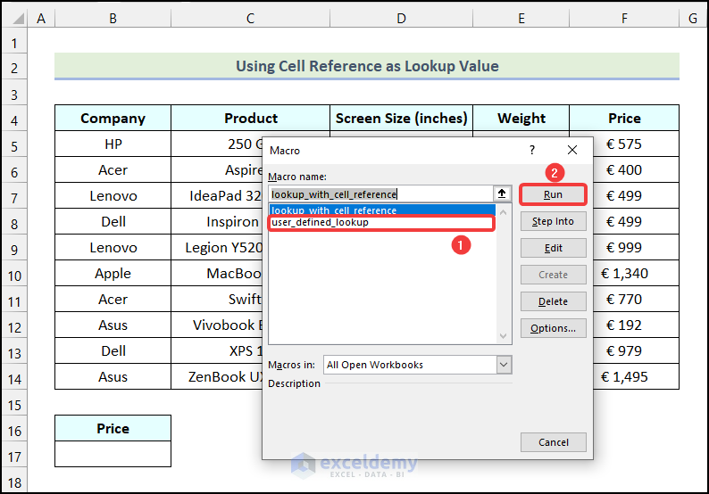
- Subsequently, use the keyboard shortcut ALT + F8 to open the Macro dialogue box.
- Following that, in the Macro dialogue box, choose the lookup_with_cell_reference option.
- Lastly, click on Run.
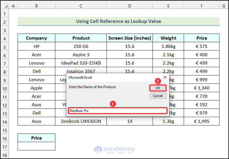
- Consequently, a dialogue box will appear on your screen. In the dialogue box, enter the name of the Product.
- Then, click OK.
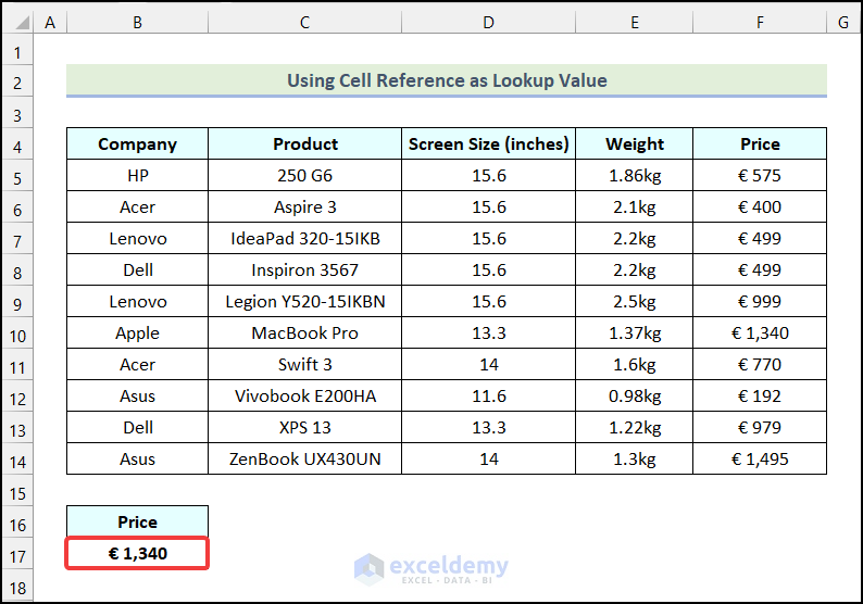
Subsequently, in cell B17, you will have the Price of the Product that you have entered in the dialogue box.
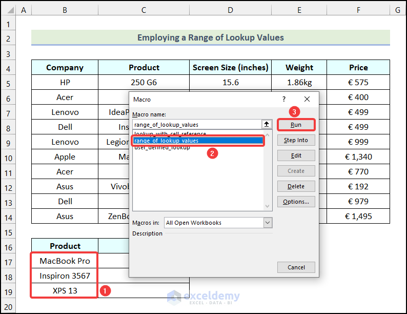
3. Employing a Range of Lookup Values
Now, we will use a range of lookup values instead of a single lookup value to find the Prices of selected laptops using the VBA Lookup function in Excel. To do this, let’s use the instructions outlined below.
Steps:
- Firstly, apply the steps mentioned in Step 01 and Step 02 of the first method.
- After that, write the following code in the newly created Module.
Sub range_of_lookup_values()
Range("C17:C19").Value = WorksheetFunction.Lookup _
(Range("B17:B19").Value, Range("C5:C14"), Range("F5:F14"))
End Sub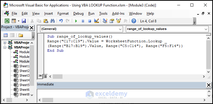
Code Breakdown
- Firstly, we created a sub-procedure named range_of_lookup_values.
- Following that, we used WorksheetFunction.Lookup Method to find the Price for the lookup value in range B17:B19 and assigned the value to range C17:C19.
- Lastly, we ended the sub-procedure.
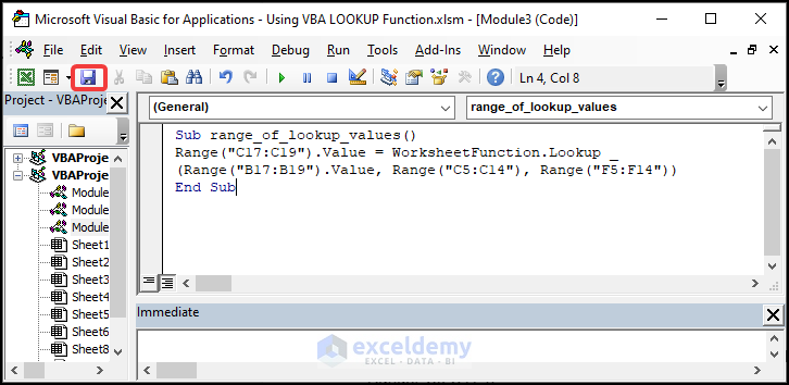
- After writing the code, click on the Save icon.
- Following that, use the keyboard shortcut ALT + F11 to return to the worksheet.
- Now, enter the names of the products in range B17:B19. This is our range of lookup values.
- After that, use the keyboard shortcut ALT + F8 to open the Macro dialogue box.
- Afterward, in the Macro dialogue box, choose the range_of_lookup_values option.
- Finally, click on Run.
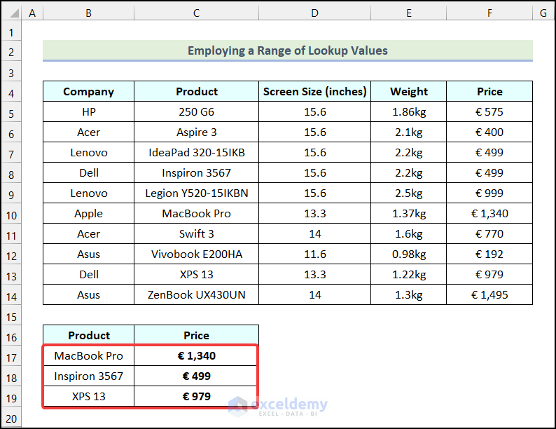
Consequently, you will have the prices for the selected lookup values as demonstrated in the following picture.
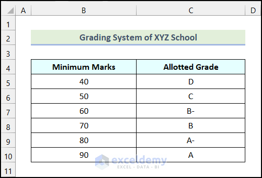
4. Calculating Grades Based on Obtained Marks
In the fourth example, we are going to calculate the Grades based on Obtained Marks by using the VBA Lookup function in Excel. Let’s say, we have the Grading System of XYZ School as our dataset. Using this dataset, we will calculate the Grades. So, let’s follow the procedure discussed in the following section.
Steps:
- Firstly, follow the steps mentioned in Step 01 and Step 02 of the first method.
- Then, write the following code in the newly created Module.
Sub calculating_grade()
Range("C14").Value = WorksheetFunction.Lookup( _
Range("B14").Value, Range("B5:B11"), Range("C5:C11"))
End Sub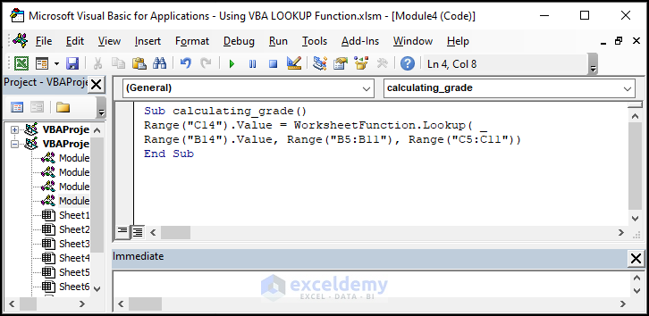
Code Breakdown
- Firstly, we created a sub-procedure named calculating_grade.
- Following that, we used WorksheetFunction.Lookup Method to find the Grade for the Obtained Marks in cell B14 and assign the value to range C14.
- Finally, we ended the sub-procedure.
- Subsequently, click on the Save icon.

- After that, use the keyboard shortcut ALT + F11 to return to the worksheet.
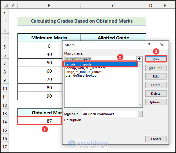
- Subsequently, insert the Obtained Marks in cell B14.
- After that, use the keyboard shortcut ALT + F8 to open the Macro dialogue box.
- Afterward, in the Macro dialogue box, choose the calculating_grade option.
- Finally, click on Run.
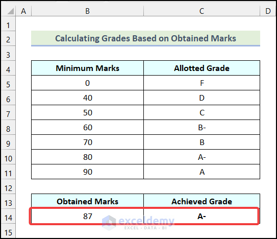
As a result, you will have the Allotted Grade based on Obtained Marks in cell C14.
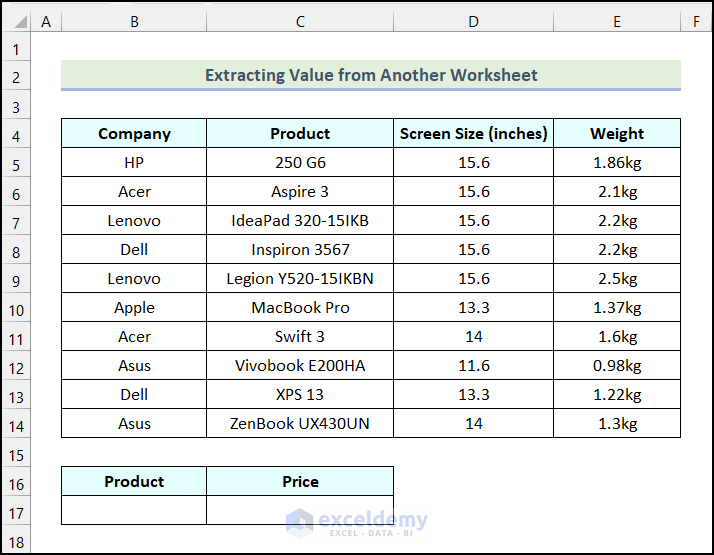
5. Extracting Value from Another Worksheet
In this section of the article, we will extract our desired value from a different worksheet. Here, we have intentionally removed the Price column from the dataset. We have used the Price column as the result vector in the previous methods. In this method, we will use the Price column from a different worksheet and use it as the result vector. Here, we will use the Price column from the worksheet named Cell Reference. Let’s use the steps mentioned in the following section.
Steps:
- Firstly, follow the steps mentioned in Step 01 and Step 02 of the first method.
- Subsequently, write the code given below in the newly created Module.
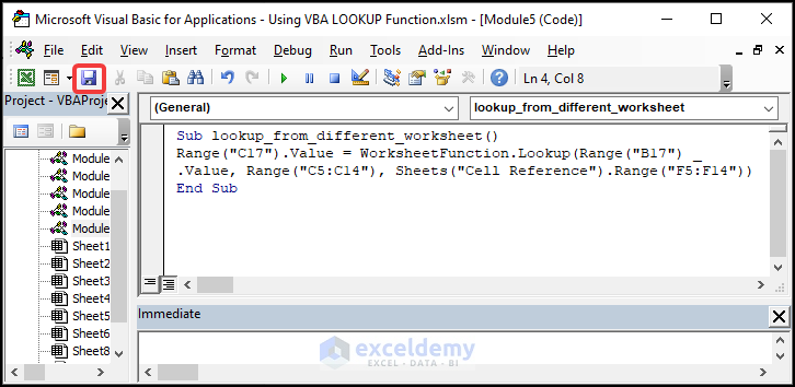
Sub lookup_from_different_worksheet()
Range("C17").Value = WorksheetFunction.Lookup(Range("B17") _
.Value, Range("C5:C14"), Sheets("Cell Reference").Range("F5:F14"))
End Sub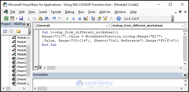
Code Breakdown
- Firstly, we created a sub-procedure named lookup_from_different_worksheet.
- Then, we used WorksheetFunction.Lookup Method to find the Price for the lookup value in cell B17 and assign the value to cell C17.
- Here, we defined the result vector from another worksheet named Cell Reference.
- Lastly, we ended the sub-procedure.
- After writing the code, click on the Save option.
- Following that, use the keyboard shortcut ALT + F11 to return to the worksheet.
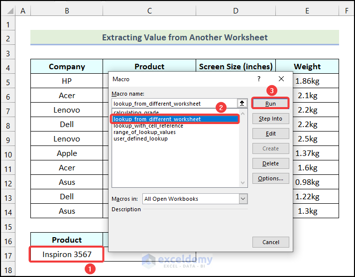
- After that, enter the name of the product in cell B17. This is our lookup value.
- After that, use the keyboard shortcut ALT + F8 to open the Macro dialogue box.
- Afterward, in the Macro dialogue box, choose the lookup_from_different_worksheet option.
- Finally, click on Run.
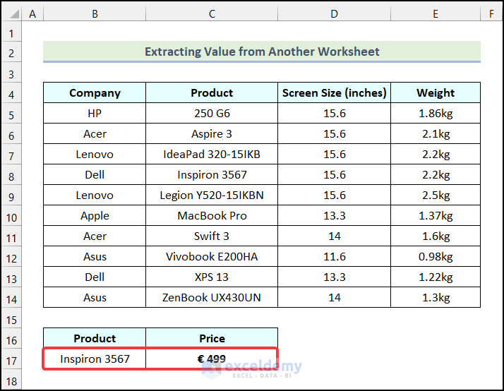
Consequently, you will have the following output in cell C17, as shown in the image below.
Read More: How to Use LOOKUP Function Among Multiple Sheets in Excel
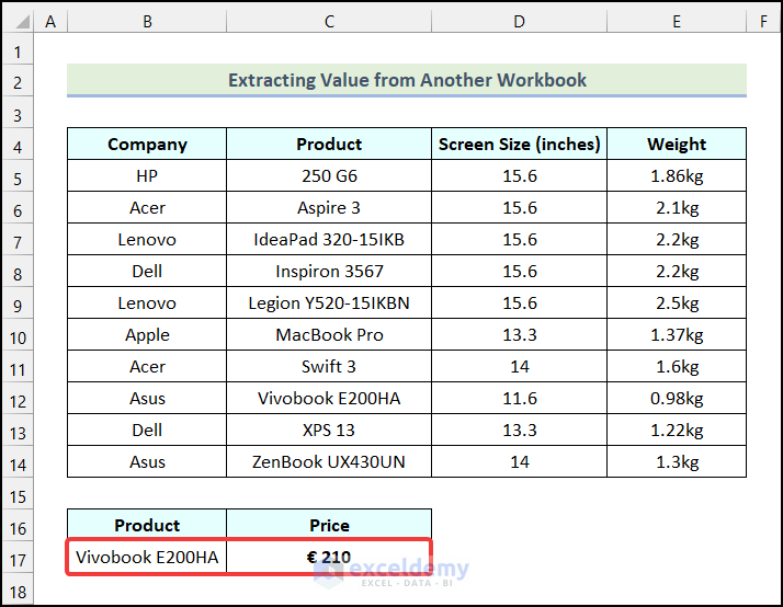
6. Finding Value from Another Workbook
In our final example, we will demonstrate how we can find and extract value from a different workbook using the VBA Lookup function in Excel. Here, we have created a new workbook named Laptop Prices and changed the values of the Price column so that we can differentiate our results from the previous workbook. We have named this worksheet as Dataset. Now let’s follow the steps outlined below.

Steps:
- Firstly, follow the steps mentioned in Step 01 and Step 02 of the first method.
- Following that, write the following code in the newly created Module.
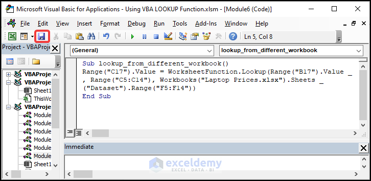
Sub lookup_from_different_workbook()
Range("C17").Value = WorksheetFunction.Lookup(Range("B17").Value _
, Range("C5:C14"), Workbooks("Laptop Prices.xlsx").Sheets _
("Dataset").Range("F5:F14"))
End Sub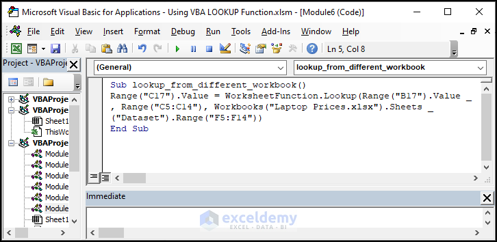
Code Breakdown
- Firstly, we created a sub-procedure named lookup_from_different_workbook.
- Then, we used WorksheetFunction.Lookup Method to find the Price for the lookup value in cell B17 and assign the value to cell C17.
- Here, we defined the result vector from another workbook named Laptop Prices. Then, we also defined the worksheet name and the range of the result vector.
- Lastly, we ended the sub-procedure.
- Now, click on the Save option.
- Subsequently, use the keyboard shortcut ALT + F11 to return to the worksheet.
- Then, enter the name of the product in cell B17. This is our lookup value.
- Now, use the keyboard shortcut ALT + F8 to open the Macro dialogue box.
- Following that, in the Macro dialogue box, choose the lookup_from_different_worksheet option.
- Lastly, click on Run.

As a result, you will have the following output in cell C17. If you look carefully, you will see that the price of Vivobook E200HA was €192 in the first workbook. But in cell C17, we have €210, which has come from the new workbook that we have created.
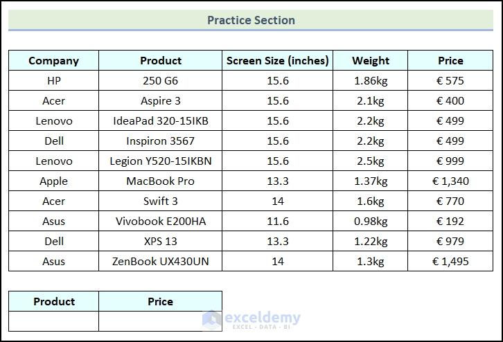
Practice Section
In the Excel Workbook, we have provided a Practice Section on the right side of the worksheet. Please practice it yourself.
Download Practice Workbook
Conclusion
So, these are the most common and effective methods you can use anytime while working with your Excel datasheet to use the VBA Lookup function in Excel. If you have any questions, suggestions, or feedback related to this article, you can comment below. Have a nice day!
<< Go Back to Excel LOOKUP Function | Excel Functions | Learn Excel
Get FREE Advanced Excel Exercises with Solutions!
