Microsoft Excel is a helpful program. You can conduct infinite operations on a dataset using Excel’s tools and capabilities. Regularly, we must search for data on other sheets. Working on one sheet and navigating to other sheets for relevant data can be time-consuming and stressful. Therefore, it is necessary to work on many sheets in Excel simultaneously. The LOOKUP function is crucial for searching and querying across several sheets in several circumstances. This article discusses two appropriate examples of utilizing the LOOKUP function to perform operations across many sheets. Be bold and review these two practical examples of using the LOOKUP Function on Multiple Sheets in Excel.
Why Do We Use LOOKUP Function?
If you enter some information in a cell in a spreadsheet, the LOOKUP function will find it and retrieve the matching data from another cell. When applied to a collection, the LOOKUP function locates the supplied value within the initial column or row and then returns a deal stored at the exact location in the final column or row.
How to Use LOOKUP Function Within Multiple Sheets in Excel: 3 Ideal Examples
To illustrate this point, let’s examine two representative datasets. The First Dataset consists of five columns titled Order ID, Product Name, Sales Rep, Delivery Date, and Status. Using the LOOKUP function, we will develop a formula to fetch a whole Order Record from another sheet titled OrderRecord when an Order ID is supplied. The Second Dataset contains four columns: Sales Rep, Salary, Salary Range, and Bonus. The columns Sales Rep and Salary comprise a table, and Similarly, the remaining two columns form a separate table. Using the LOOKUP function, we will create two formulas to determine a sales representative’s Bonus and return the data to the SalaryBonus sheet. It is essential to note that both datasets belong to the Dataset sheet.
I’ve also been using Microsoft Excel 365 to compose this post. You are free to select the version that best meets your needs, and whichever option you choose is acceptable to us.
1. Utilize LOOKUP Function Within Multiple Sheets to Find Order Records in Excel
The LOOKUP command enables the user to enter a value in one column or row and has it matched to some other field or column’s value. Throughout this context, we will build a system that fetches the whole record of a particular order from different sheets if we provide an Order ID. To complete the work with the assistance of the LOOKUP function, adhere to the guidelines below.
STEPS:
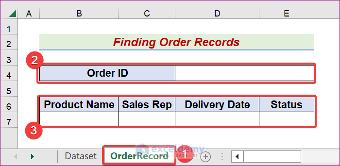
- First, select the OrderRecord sheet as the Active sheet.
- Second, create a search box named Order ID.
- Third, choose four columns titled: Product Name, Sales Rep, Delivery Date, and Status in the B6:E7 range.
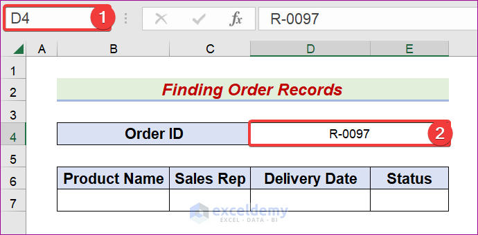
- After that, pick the D4 cell and input the desired Order ID from the Dataset, in this case, R-0097.
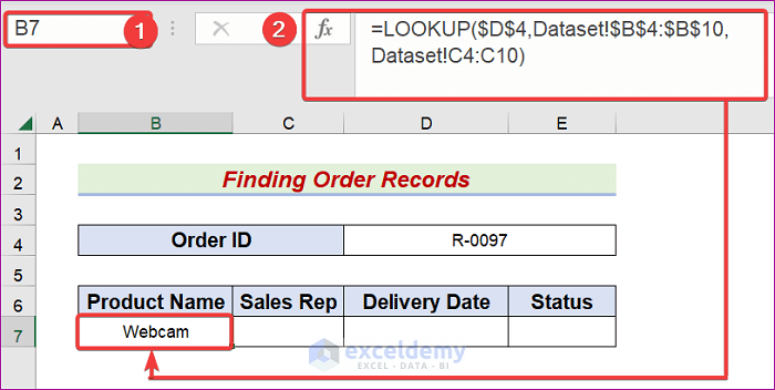
- Later, select the B7 cell.
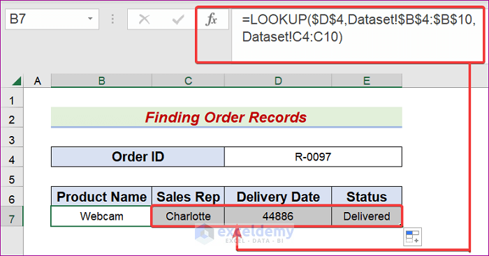
- Next, type the following equation in the Formula bar.
=LOOKUP($D$4,Dataset!$B$4:$B$10,Dataset!E4:E10)
- Afterward, hit the Enter or Tab key to see the outcome like the below one.
- Now, we must use the same formula for other cells.
- To attain this, drag the AutoFill Handle icon to cell E7.
- Subsequently, we will see the intended result.
- Now, choose the D7 cell and go to the Home tab.
- Later, select Date as the Number Format.
- Consequently, we will get the desired output like the following.

=LOOKUP($D$4,Dataset!$B$4:$B$10,Dataset!E4:E10)
For this formula to make sense, you need to know how to use the following Excel function:
LOOKUP Function
- LOOKUP($D$4,Dataset!$B$4:$B$10,Dataset!E4:E10)
The LOOKUP function utilizes an item from one range, finds its equivalent in another, and returns it. We must put an Exclamation mark between the sheet’s name and the range to refer to data or cells in other sheets. In this example, by involving the LOOKUP function, we find Webcam.
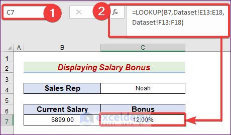
2. Display Salary Bonus Employing LOOKUP Function Throughout Different Sheets in Excel
Here, we will find out the Bonus of Sales Reps according to their Current Salary utilizing the LOOKUP function. Follow the directions below to successfully finish the work with the help of the LOOKUP function.
STEPS:
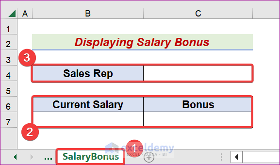
- First, set the SalaryBonus sheet as the Active sheet.
- Second, create a search box called Sales Rep.
- Third, choose two columns, Current Salary, and Bonus, in the range B6:C7.
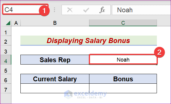
- After that, select the C4 cell and input the desired Sales Rep name.
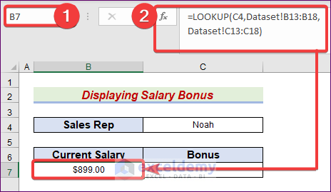
- Later, pick the B7 cell and input the below formula in the Formula bar.
=LOOKUP(C4,Dataset!B13:B18,Dataset!C13:C18)
- Next, hit Enter to see the intended outcome.
- Likewise, select the C7 cell and write the equation below in the Formula bar.
=LOOKUP(B7,Dataset!E13:E18,Dataset!F13:F18)
- Lastly, hit the Enter or Tab key to get the intended result, like the following.
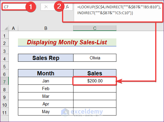
3. Find Out Monthly Sales-List Based on Employee Name Using LOOKUP Function in Excel
Throughout this context, we will find the Monthly Sales-List of Sales Reps according to their name utilizing the LOOKUP and INDIRECT functions. To illustrate this point, let’s examine some sheets of representative datasets titled Jan, Feb, March, April, and May. All these sheets contain two columns named Sales Rep and Sales. Follow the directions below to successfully finish the work with the help of the LOOKUP function.
3.1 Apply Vector Form of LOOKUP Function Among Multiple Sheets
To get information from a specific location in a table, the Vector version of the LOOKUP function first searches a single row or column for the value you specify.
STEPS:
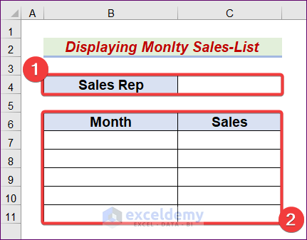
- First, create a search box named Sales Rep.
- Second, build two columns titled Month and Sales in the range B6:C11.

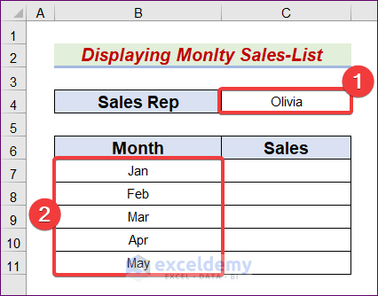
- Third, insert the employee’s name and the months.

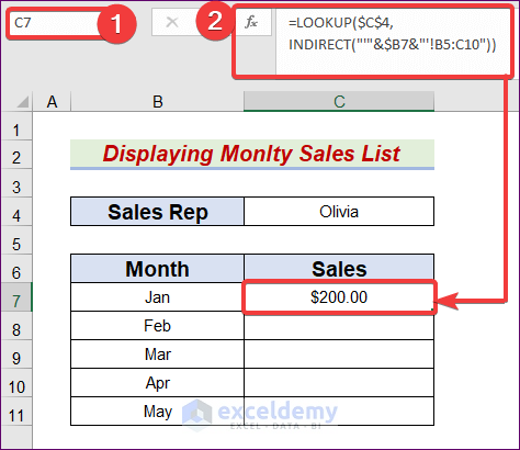
- After that, select the C7 cell and input the following equation.
=LOOKUP($C$4,INDIRECT("'"&$B7&"'!B5:B10"),INDIRECT("'"&$B7&"'!C5:C10"))
- Later, press the Enter or Tab key to see the outcome.
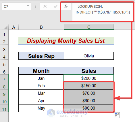
- At this point, drag the AutoFill Handle icon and move it to C11.
- Consequently, the desired result will display like the below one.
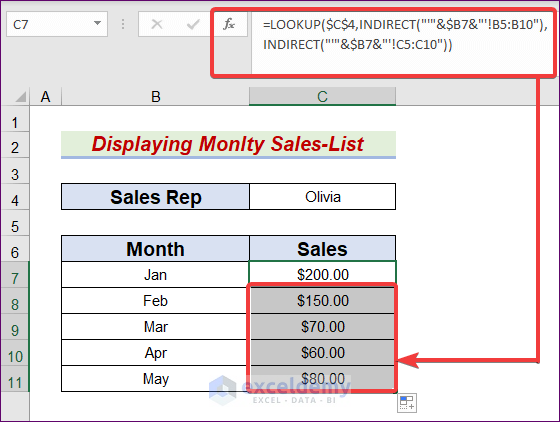
=LOOKUP($C$4,INDIRECT("'"&$B7&"'!B5:B10"),INDIRECT("'"&$B7&"'!C5:C10"))
To understand this formula, you must be familiar with the following Excel functions:
LOOKUP and INDIRECT Functions
- INDIRECT(“‘”&$B7&”‘!B5:B10”),INDIRECT(“‘”&$B7&”‘!C5:C10”)
You can get a range reference back using the INDIRECT function in Excel. To refer a data or cells in other sheets, we must use an Exclamation sign between the sheet name and range. In this demonstration, by involving the INDIRECT function, we find {“Charlotte”;”Elijah”;”Emma”;”Noah”;”Oliver”;”Olivia”} as lookup_vector and get {110;215;74;65;103;200} as [result_vector].
- LOOKUP($C$4,INDIRECT(“‘”&$B7&”‘!B5:B10”),INDIRECT(“‘”&$B7&”‘!C5:C10”))
In this context, by utilizing the LOOKUP function, we find 200.
3.2 Employ Array Form of LOOKUP Function in Excel
The Array version of the LOOKUP function searches for the supplied value in the first column or row of an array and produces an output in the exact location in the array’s final columns or rows. If the item is found, the array version of LOOKUP delivers it.
STEPS:
- To begin, make a search field titled Sales Rep.
- Second, build two columns in the range B6:C11 labeled Month and Sales.
- Later, provide the employee’s name and months.
- Presently, select the C7 cell and then enter the following equation:
=LOOKUP($C$4,INDIRECT("'"&$B7&"'!B5:C10"))
- Press the Enter or Tab key to view the result.
- At this stage, move the AutoFill Handle symbol to cell C11 using the drag handle.
- As a result, the intended outcome will appear as shown below.
Read More: How to Use VBA Lookup Function in Excel
Things to Keep in Mind
The Order ID column and the Sales Rep column are intentionally sorted. We did this because the lookup_vector must always be provided in ascending order when working with the LOOKUP function. Otherwise, the LOOKUP feature will malfunction.
- Sort the lookup_vector in ascending order.
Download Practice Workbook
If you would like a free copy of the illustrated workbook that we covered during the presentation, please click on the link that can be found just below this section.
Conclusion
If you follow the examples we just went through, you will be able to use the LOOKUP Function within Multiple Sheets in Excel going forward. Let us know if you have any other ideas or ways to accomplish the task or if you’re looking for something different to try. If you have any questions or comments, please submit them in the area below.
<< Go Back to Excel LOOKUP Function | Excel Functions | Learn Excel
Get FREE Advanced Excel Exercises with Solutions!
