Method 1 – Using Fuzzy Lookup Add-In
Step-01: Creation of Two Tables for Fuzzy Lookup Excel
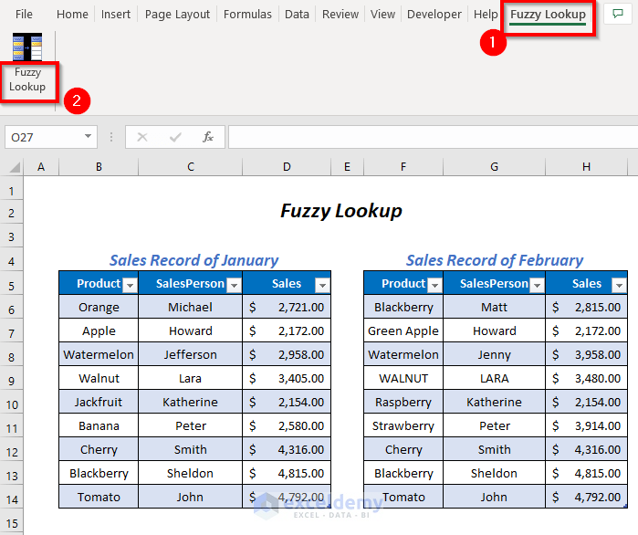
Before using the Fuzzy Lookup option we have to convert the following two data ranges into two different tables.
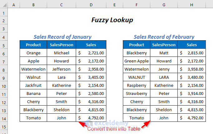
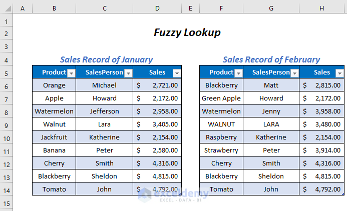
Following the article “How to Make a Table in Excel” we have converted the ranges into these tables.
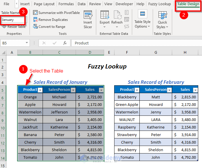
Rename these tables.
➤ Select the table for Sales Record of January and then go to Table Design Tab >> rename the Table Name as January.
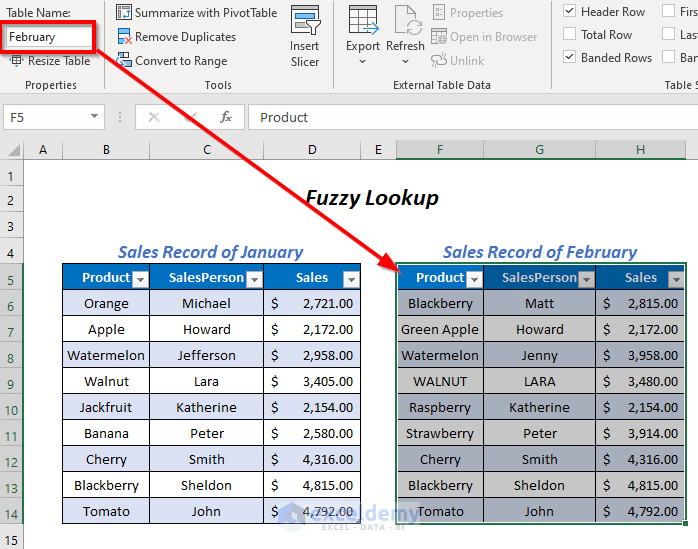
Rename the Sales Record of February table as February.
Step – 02: Creating Fuzzy Lookup with Fuzzy Lookup Excel Add-In
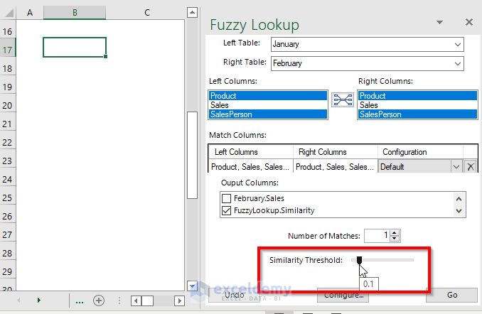
➤ Go to Fuzzy Lookup Tab >> Fuzzy Lookup Option.
Get a Fuzzy Lookup portion on the right pane.
➤ Select the cell where you want your output comparison table.
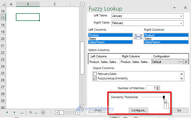
➤ Choose the Left Table as January and the Right Table as February.
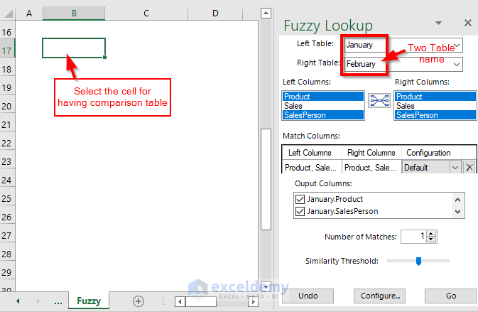
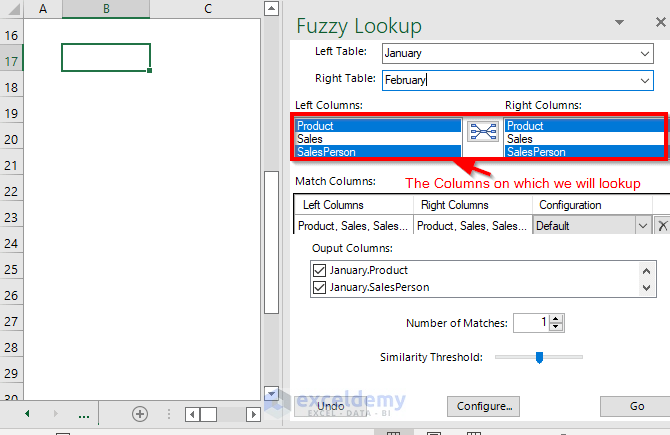
Select the columns on which we want this comparison. We want this comparison on the basis of the Product column and the SalesPerson column, so these columns are selected in the Left Columns and Right Columns boxes.
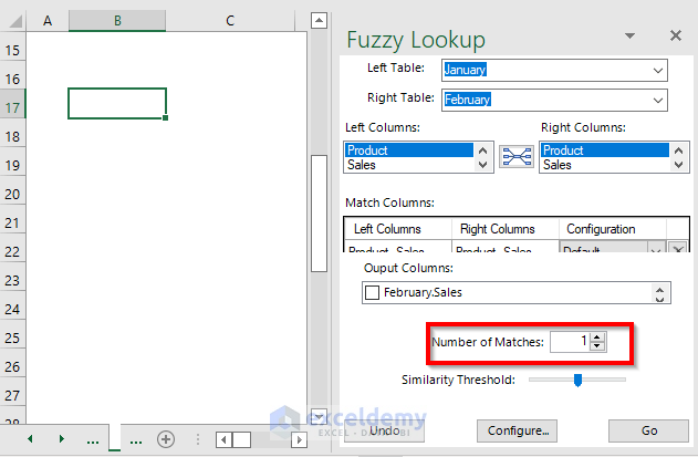
As Output Columns select the January.Product and January.SalesPerson from the January table and,
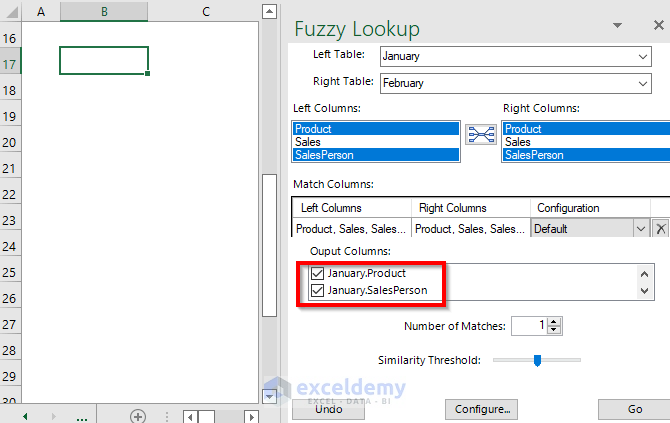
February.Product and Febuary.SalesPerson from the February table and finally,
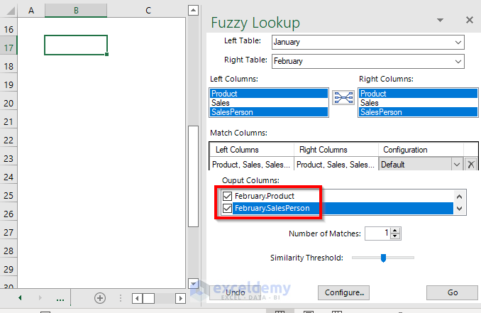
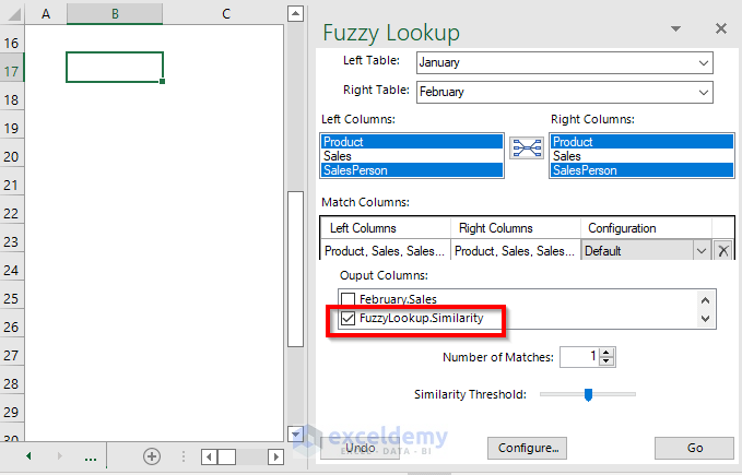
Select the FuzzyLookup.Similarity for getting the percentage indication of similarities.
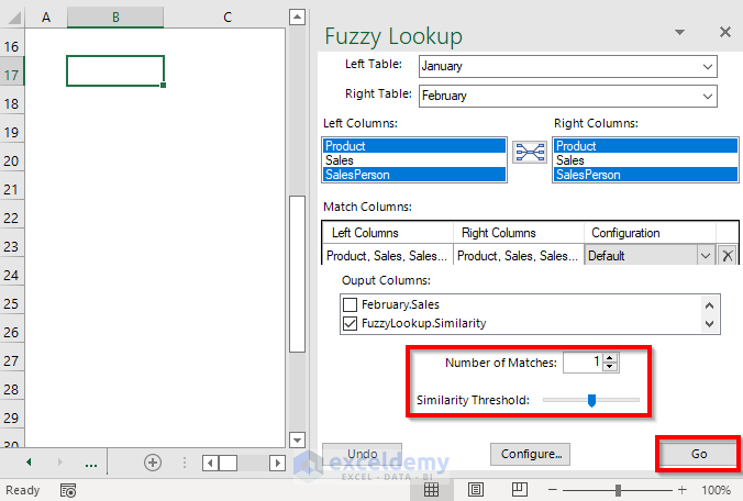
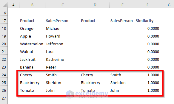
We selected the Number of Matches as 1 and the Similarity Threshold as 0.51 and then pressed Go.
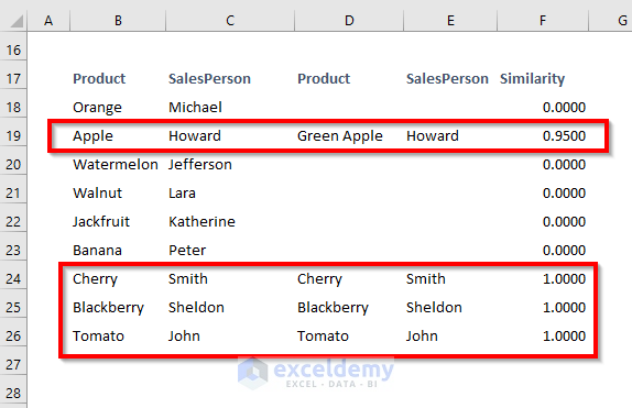
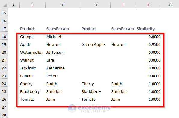
We got matches for the Products Apple and Green Apple for the SalesPerson Howard and for Cherry, Blackberry, and Tomato which are fully matched as the similarity is 100%.
Effects of Changing Number of Matches and Similarity Threshold
Number of Matches:
For selecting the Number of Matches as 1,
We are getting the following comparison table where we have one similarity for each product, but we had Blackberry 2 times in the February table with different SalesPersons.
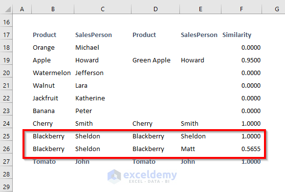
If you select the Number of Matches as 2,
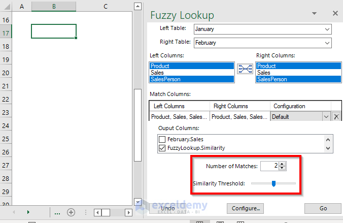
You will get the matching results for these two Blackberry products with the SalesPerson Sheldon and Matt.
Similarity Threshold:
Its range is between 0 and 1, and to move from the lower range to the higher range, we will move from partial match to exact match.
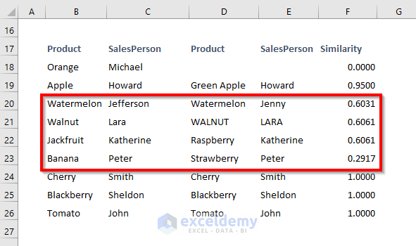
Try with a Similarity Threshold of 0.1.
We are getting the similarities from 20% to 100%.
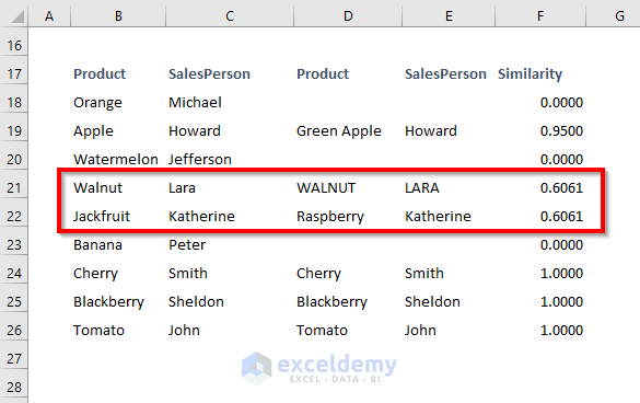
For selecting the Similarity Threshold as 0.4,

The similarity range is from 60% to 100%.
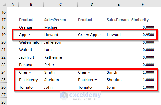
When we have selected the Similarity Threshold range as 0.84,

Then the similarity range is from 90% to 100%.
For selecting the highest Similarity Threshold range like 1,
Then you will get only the exact matches as the similarity range is 100%.
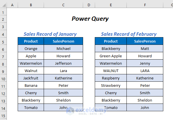
Method 2 – Power Query Fuzzy Matching Option
Step-01: Creation of Two Queries
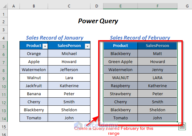
For comparing the Product and SalesPerson columns of the January and February sales records, we will convert these two ranges into queries.
➤ Go to Data Tab >> From Table/Range option.
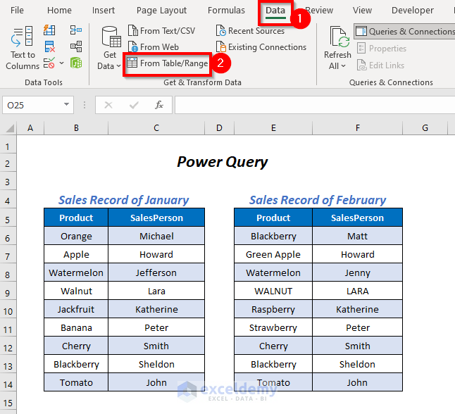
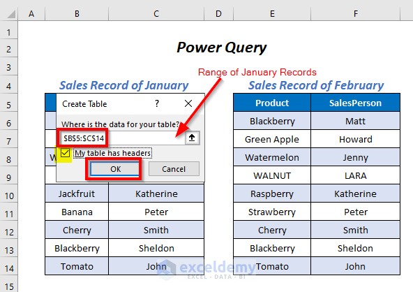
The Create Table wizard will pop up.
➤ Select the range of your data table (we are selecting the data range of the Sales Record of January)
➤ Check My table has headers option and press OK.
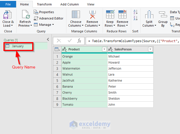
A Power Query editor will open up.
➤ Rename the query as January.
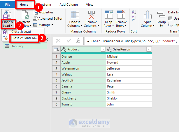
We will import this data as a connection only.
➤ Go to Home Tab >> Close & Load Dropdown >> Close & Load To option.
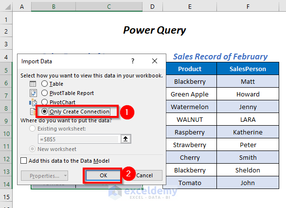
The Import Data dialog box will appear.
➤ Click on the Only Create Connection option and press OK.
Create a query named February for the dataset Sales Record of February.
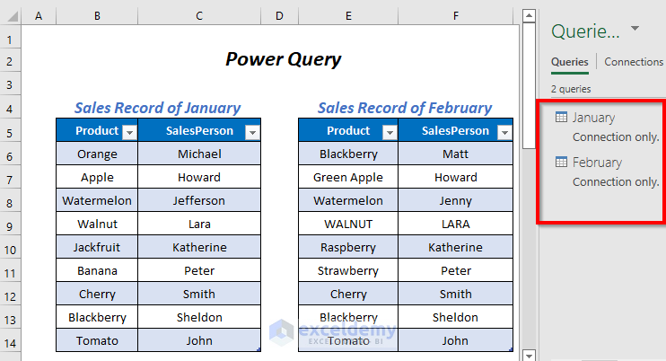
We can see the names of the two queries in January and February that we created in this step.
Step-02: Combining Queries for Fuzzy Lookup Excel
We will combine the queries of the previous step to match the data of these queries.
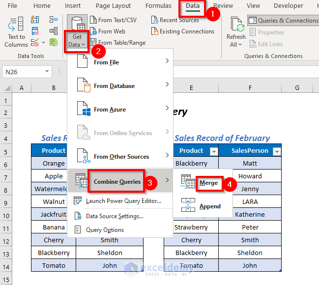
➤ Go to Data Tab >> Get Data Dropdown >> Combine Queries Dropdown >> Merge Option.
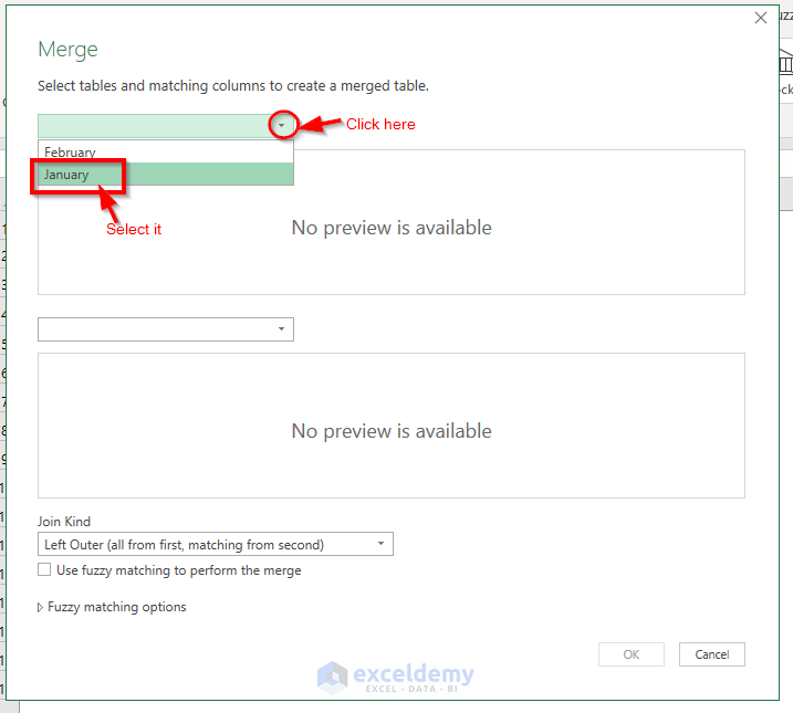
The Merge wizard will pop up.
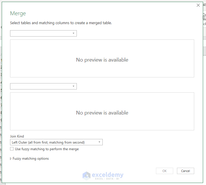
➤ Click the dropdown of the first box and then select the January option.
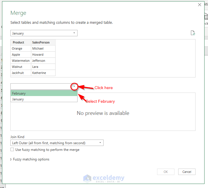
➤ Select the dropdown of the second box and then select the February option.
Select the columns of the two queries by pressing CTRL with a Left-click at a time on the basis of which we want to match our data.
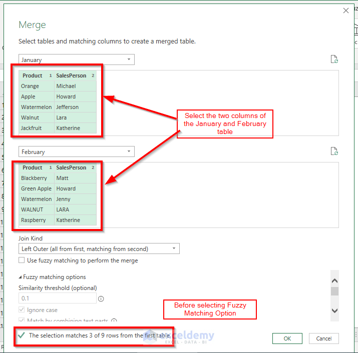
See that it has found 3 rows matching from 9 rows.
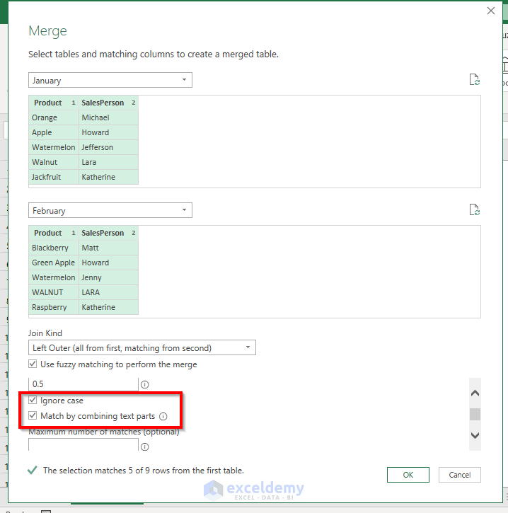
Step-03: Using the Fuzzy Matching Option for Fuzzy Lookup Excel
Use the Fuzzy Matching option to perform the partial matching beside the exact matches.
➤ Check the Use fuzzy matching to perform the merge option and then select the Similarity threshold as 0.5 for this option.
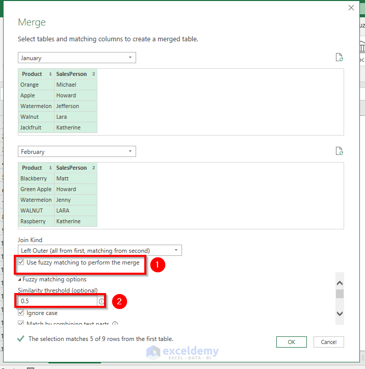
➤ Select the Ignore case option and the Match by combining text parts option.
We selected the Maximum number of matches as 1 and pressed OK.
See the matching number has been increased from 3 to 5.
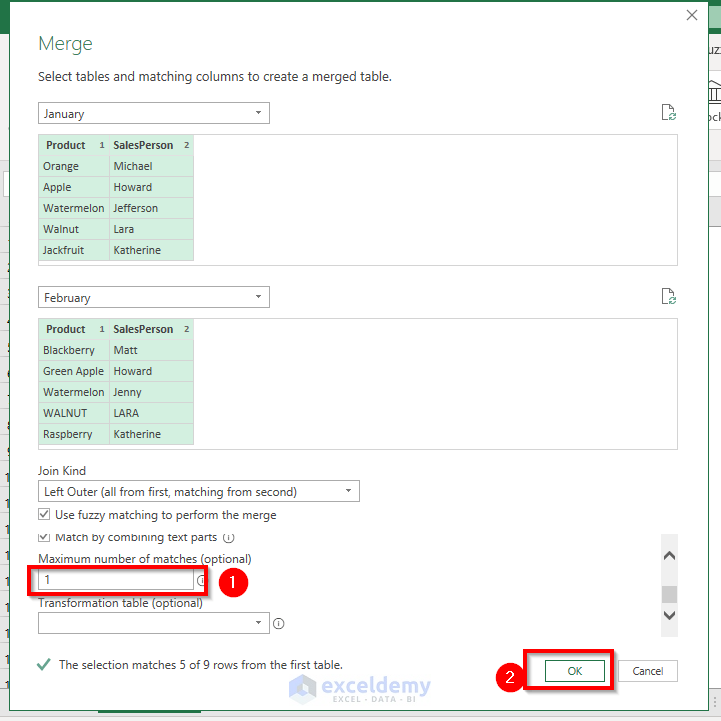
You will be taken to the Power Query Editor window.
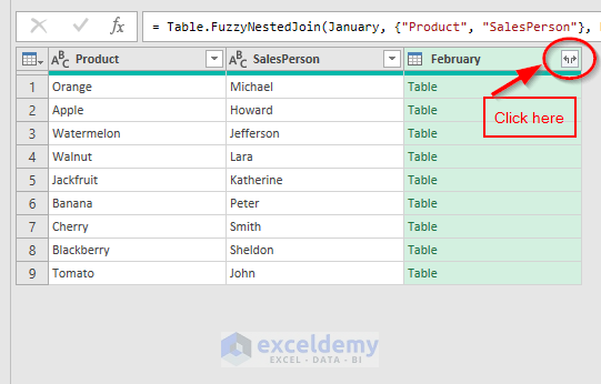
See the first two columns from the January query but the columns of the February query are hidden. So, we have to expand this February column.
➤ Click on the indicated sign beside February.
➤ Select the Expand option and press OK.
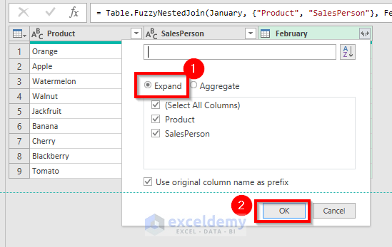
We can see the matches of the two queries properly.

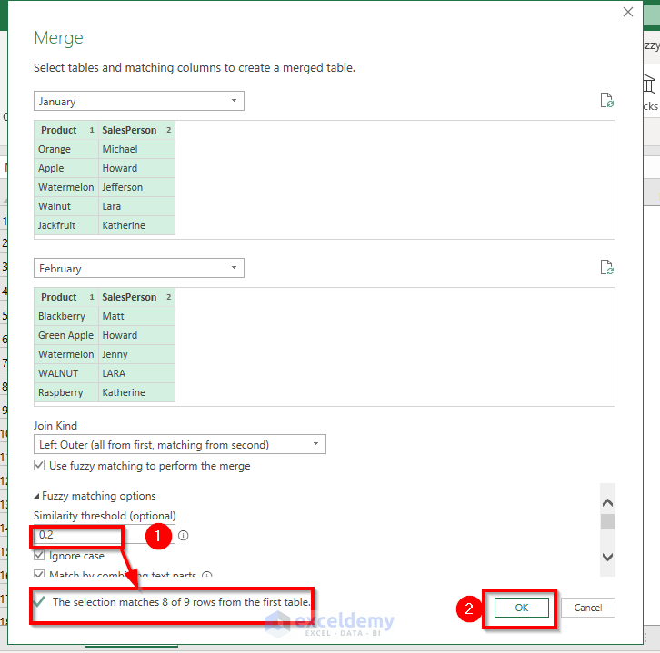
Effects of Changing Similarity Threshold
If we change the Similarity threshold from 0.5 to 0.2, then we will have 8 matches in the place of 5 matches.
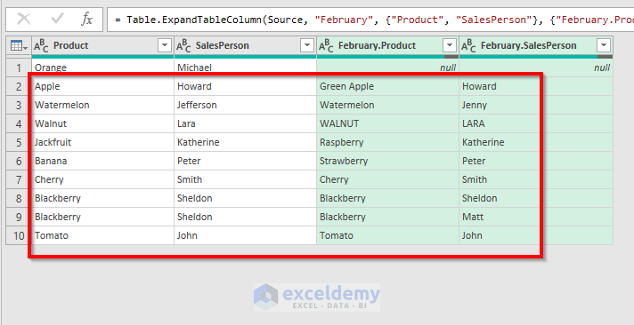
After pressing OK, we can see that, the other rows are partially similar to each other except for the first row.
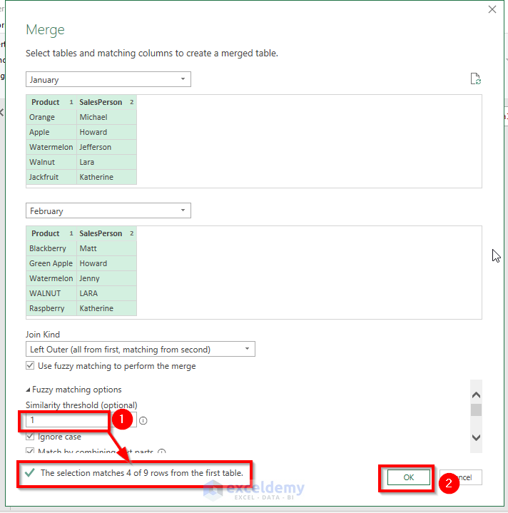
If we select the Similarity threshold from 0.2 to 1, we will have 4 matches instead of 8 matches.
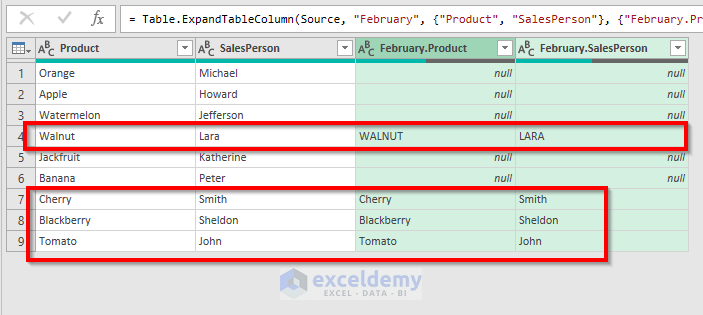
The exact matches ignore cases only. We are having the results this time.
Things to Remember
The built-in lookup functions like the VLOOKUP function, HLOOKUP function are useful for exact matching cases, but for finding approximate matches according to our wish we can use the Fuzzy Lookup add-in of Excel.
To produce different results for matching cases, you can change the Number of Matches and Similarity Threshold parameters as per your necessity.
Download Practice Workbook
<< Go Back to Lookup | Formula List | Learn Excel
Get FREE Advanced Excel Exercises with Solutions!
