Method 1 – Using an Array Formula to Lookup Multiple Values in Excel
The VLOOKUP Function can only return a single match.
We can use an array formula with one of the following functions:
- IF – It outputs one value if the condition is satisfied and another value if the condition is not satisfied.
- SMALL – It returns the array’s lowest value.
- INDEX – Gives an array element depending on the rows and columns provided by you.
- ROW – It provides you with the row number.
- COLUMN – It gives you the number of the column.
- IFERROR – detect errors.
When applying an array formula in versions of Excel other than Excel 365, you need to use Ctrl + Shift + Enter instead of Enter.
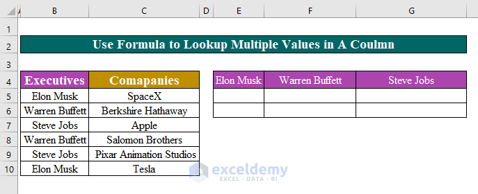
Case 1.1 – Lookup Multiple Values in A Row
We have a few names of executives who run multiple companies in column B. We’ll compile a list of all businesses (from C) run by a specific person.
Steps:
- In an empty row, provide a list of unique names. The names are entered in cells B13:B15 in this example.
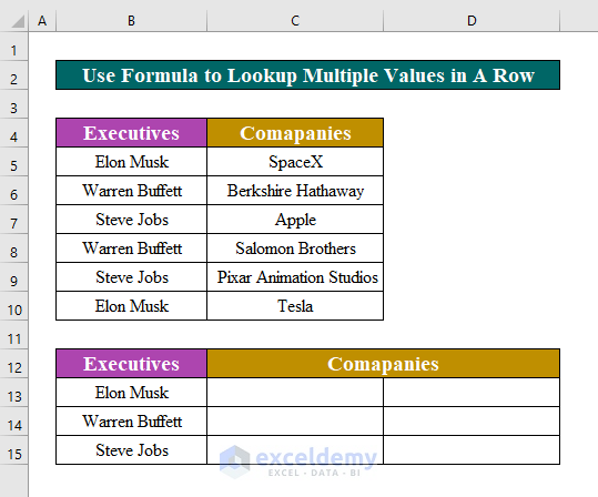
- Enter the following formula in the cell C13.
=IFERROR(INDEX($C$5:$C$10, SMALL(IF($B15=$B$5:$B$10, ROW($C$5:$C$10)-4, " "), COLUMN()-2)), " ")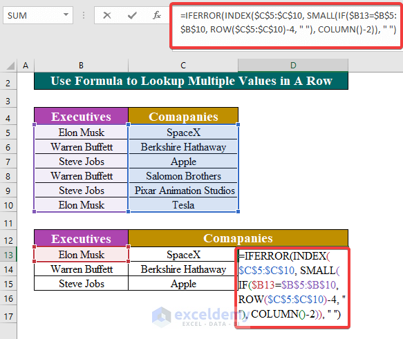
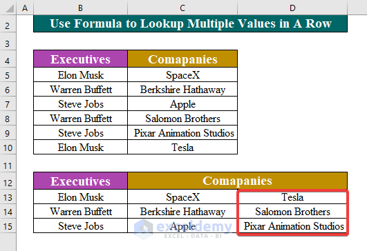
- Use AutoFill to see the results.
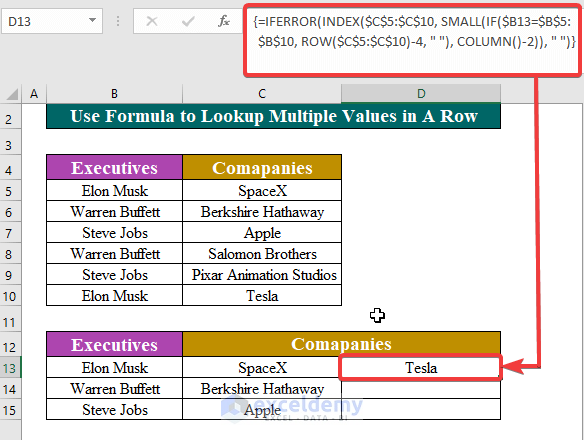
- Here’s the result.
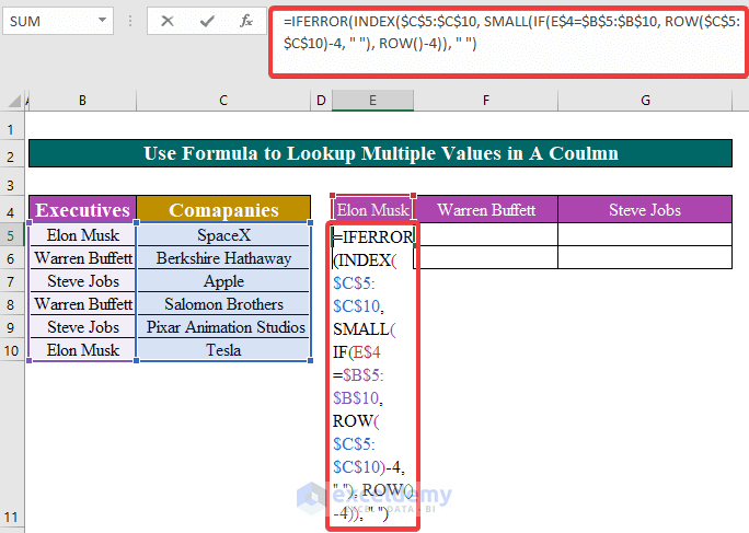
Case 1.2 – Lookup Multiple Values in a Column in Excel
We modified the result table.
Steps:
- Enter a list of unique names in and empty row such as cells E4:G4.
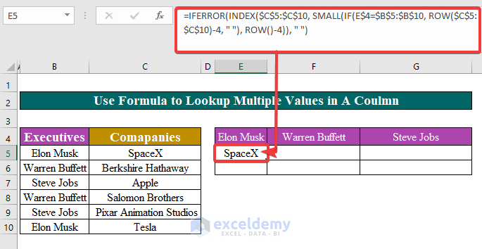
- Apply the following formula in cell E5.
=IFERROR(INDEX($C$5:$C$10, SMALL(IF(E$4=$B$5:$B$10, ROW($C$5:$C$10)-4, " "), ROW()-4)), " ")- Press Ctrl + Shift + Enter.
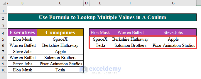
- Fill the other cell with the AutoFill handle tool.
- Here’s the result.
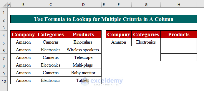
Method 2 – Searching for Multiple Values in Excel Based on Multiple Criteria
We have a data set of Amazon bestselling products under specific categories in different columns. We’ll get a product under a certain category.
We will use the following array formula:
IFERROR(INDEX(return_range, SMALL(IF(1=((–(lookup_value1=lookup_range1)) * ( –(lookup_value2=lookup_range2))), ROW(return_range)-m,””), ROW()-n)),””)
Lookup_value1 is the first lookup value in cell F5
Lookup_value2 is the second lookup value in cell G5
Lookup_range1 is the range where lookup_value1 will be searched (B5:B10)
Lookup_range2 is the range where lookup_value2 will be searched (C5:C10)
Return_range is the range from where the result will be given.
m is the row number of the first cell in the return range minus 1.
n is the row number of the first formula cell minus 1.
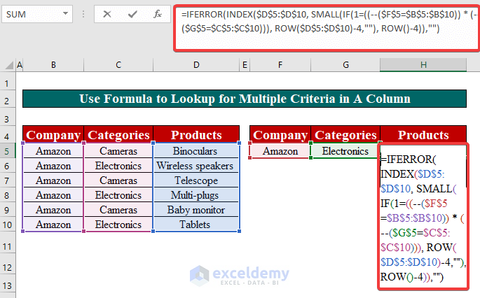
Case 2.1 – Look up Multiple Matches in a Column
Steps:
- In cell H5, insert the following formula.
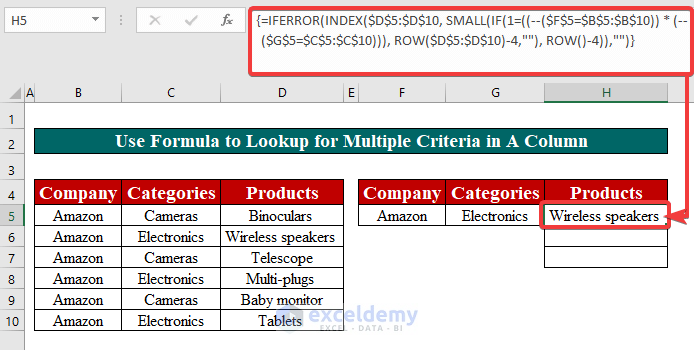
=IFERROR(INDEX($D$5:$D$10, SMALL(IF(1=((--($F$5=$B$5:$B$10)) * (--($G$5=$C$5:$C$10))), ROW($D$5:$D$10)-4,""), ROW()-4)),"")- Press Ctrl + Shift + Enter to apply the formula
- It will show the value in the below screenshot.
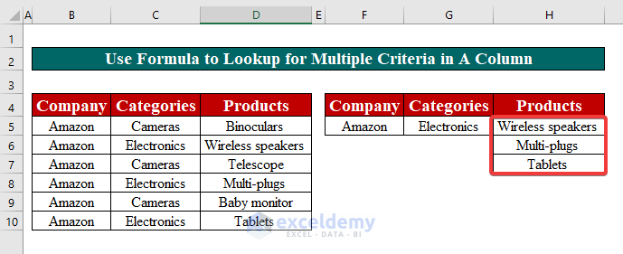
- Apply the same formula to the rest of the cells.
Note. Because our return range and formula range both begin in row 5, both n and m are equal to “4” in the example above. These may be different numbers in your worksheets.
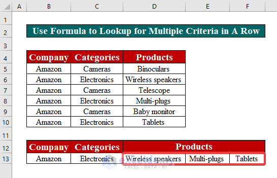
Case 2.2 – Look up Multiple Matches in a Row
We can modify the table for a horizontal layout.
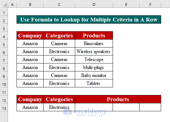
Steps:
- In cell D13, enter the following formula:
=IFERROR(INDEX($D$5:$D$10, SMALL(IF(1=((--($B$13=$B$5:$B$10)) * (--($C$13=$C$5:$C$10))), ROW($D$5:$D$10)-4,""), COLUMN()-3)),"")- Press Ctrl + Shift + Enter.
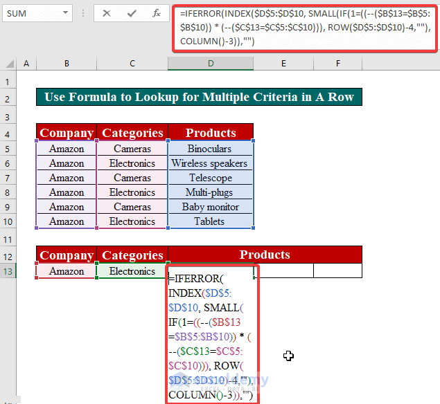
- Use AutoFill to fill in the other cells.
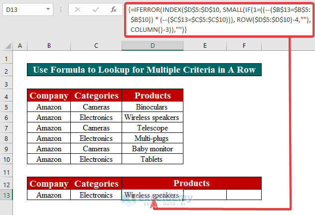
- Here’s the result.
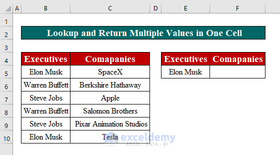
Method 3 – Returning Multiple Values in One Cell After a Lookup
This method uses functions only available in Excel 365 at the time of writing.
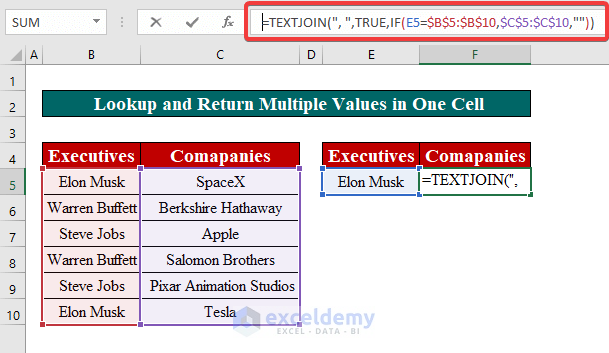
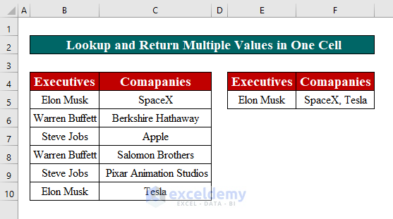
We have a data set with the names of the executives in column B and the companies they own in column C. For each person, we want to look up which companies they own in a single list (separated by a comma) in cell F5.
Steps:
- Insert the following formula in cell F5.
=TEXTJOIN(", ",TRUE,IF(E5=$B$5:$B$10,$C$5:$C$10,""))- Hit Ctrl + Shift + Enter.
- Here are the results.
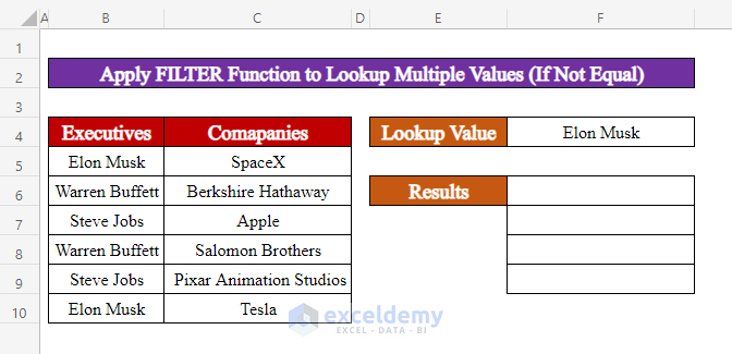
Method 4 – Applying the FILTER Function to Lookup Multiple Values in Excel
The FILTER Function is available in Excel 365. It has the following syntax.
FILTER(array, include, [if_empty])
Array (required) – the value range or array that you wish to filter.
Include (required) – the criterion provided in the form of a Boolean array (TRUE and FALSE values). It must have the same height (when data is in columns) or width (when data is in rows) as the array parameter.
If_empty (optional) – When no items fit the criterion, this is the value to return.
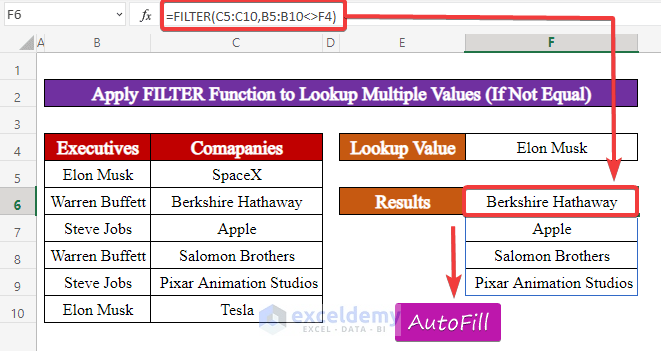
Case 4.1 – IF Not Equal
We’ll fetch the company’s names that do not belong to Elon Musk.
Steps:
- In cell F6, input the following formula:
=FILTER(C5:C10,B5:B10<>F4)- Press Enter.
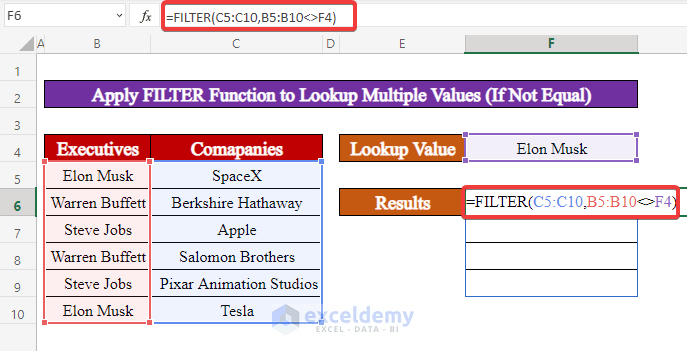
- Use the AutoFill Tool to fill the required field.
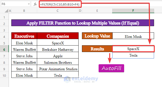
Case 4.2 – IF Equal
We’ll get the names of the companies that belong to Elon Musk.
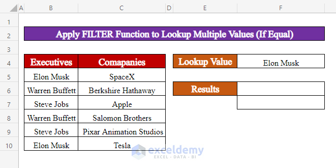
Steps:
- Insert the following formula in cell F6:
=FILTER(C5:C10,B5:B10=F4)- Hit Ctrl + Shift + Enter.
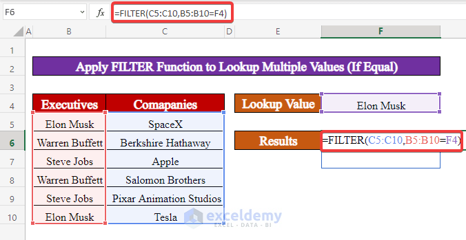
- Apply the AutoFill Handle Tool to fill the cells.
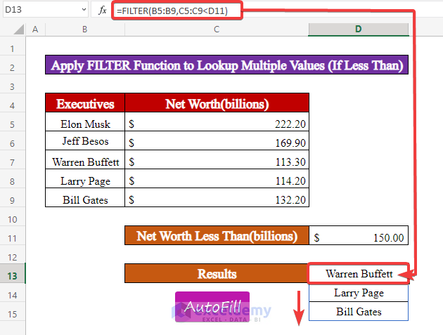
Case 4.3 – IF Less Than
We have a list of net worths and want to fetch names with net worths less than $150B.
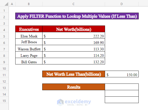
Steps:
- Insert the following formula in cell F6:
=FILTER(C5:C10,B5:B10<F4)- Press Ctrl + Shift + Enter.
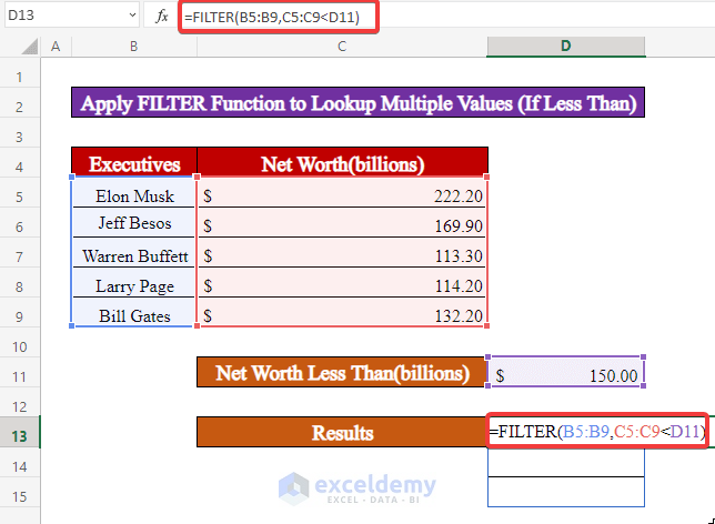
- Apply the AutoFill tool to fill the cells.
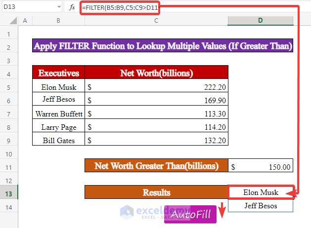
Case 4.4 – IF Greater Than
We’ll fetch net worths greater than $150B.
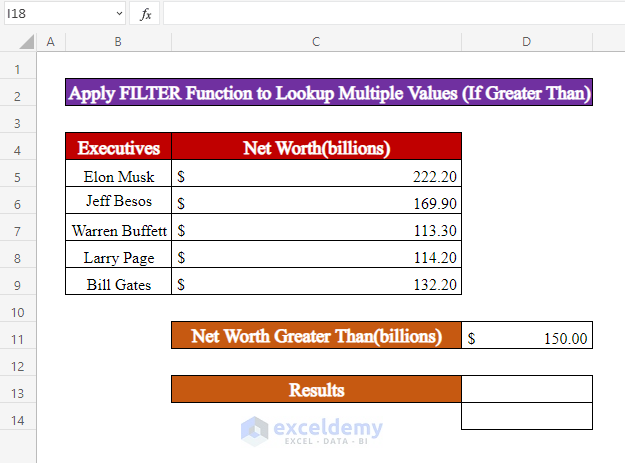
Steps:
- In cell F6, insert the following formula:
=FILTER(C5:C10,B5:B10>F4)- Hit Ctrl + Shift + Enter.
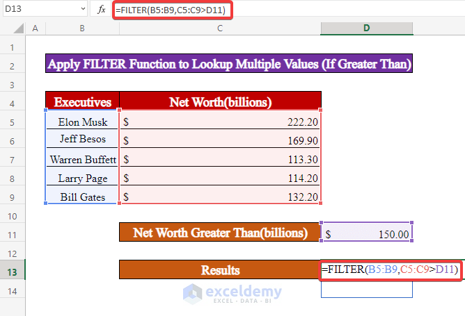
- Apply the AutoFill tool to fill the cells.
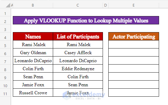
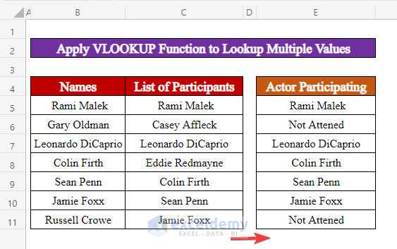
Method 5 – Applying the VLOOKUP Function to Lookup Multiple Values
We have a list of actor names in one column and a list of participants of an event in another. We’ll fetch the list of participating actors by looking up each value from one list in another.
The syntax of the VLOOKUP Function is as follows.
=VLOOKUP(lookup_value,table_array,col_index_num,[range_lookup])
Lookup_value is the reference value, which can be a text, a numerical string, or a cell whose value you want to reference.
Table_array is the whole data table including its whole. As a result, the reference value you’re seeking should be in column 1 of this table, so Excel can proceed to the right and look for the return value.
Col_index_num is the number of the column in which the return value is found. This number starts at 1 and increases as the number of columns in your table grows.
[range_lookup] is the fourth argument in brackets because it isn’t required for this function to work. In Excel syntax, brackets indicate that an argument is optional. If you don’t fill in this value, Excel defaults to TRUE (or 1), indicating that you’re seeking a close match to your reference value rather than an exact match.
Note. For text searches, using TRUE as the last argument is not advised.
Steps:
- In cell E5, insert the following formula:
=IFERROR(VLOOKUP(B5,C:C,1,FALSE),"Did Not Attend")- Press Ctrl + Shift + Enter.
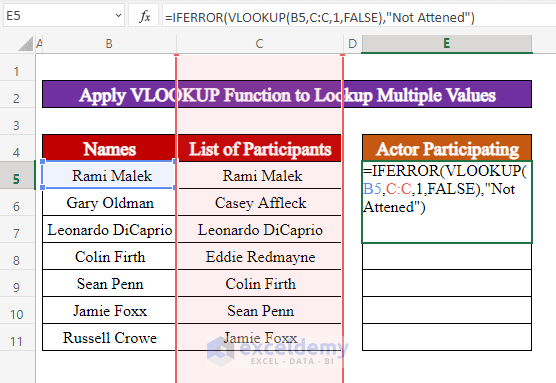
- Use AutoFill to fill the cells.
Download the Practice Workbook
<< Go Back to Lookup | Formula List | Learn Excel
Get FREE Advanced Excel Exercises with Solutions!

Hi,
your work is great. have tried to follow your lessons but seems the examples do not fit my need and I am kind of stuck trying to figure out the right formula that will give me correct result.
I would like to know who should be the receiver if the the fruit is given (1st criteria) and the number of pieces (2nd criteria) is known.
mango apple grapes strawberry
paul 1 2 4 5
james 2 3 5 6
kent 3 4 6 7
ralph 4 5 7 8
1st Criteria: fruit = grapes
2nd Criteria: number = 6
Result: name = ??? (kent)
Thanks in advance and more power to you.
Greetings,
According to your query, the ExcelDemy team has created an Excel file with the solution. Please provide your email address here, we will send it to you in no time.
Otherwise, you can just follow the procedures as we have proceeded.
Step 1:
a. Our data set range is B4:F8.
b. The names of the fruits range is C4:F4.
c. Names of people range is B5:B8.
Step 2:
a. In cell C11, create a drop-down list with the range C4:F4.
b. Give a named range for the numbers of each fruit with its name (Ex: Named range = Mango for C5:C8).
c. Create another dropdown list dependant to the cell C11. Use the following formula in the Data Validation box from the Data tab to do this.
Step 3:
a. In cell C15, insert the following formula for Mango.
b. AutoFill the formula with dragging right for three cells for more three fruits.
Step 4:
a. Now, you are done, select any name (Grapes) from the first drop-down list.
b. Then, select the number (6).
c. It will result in the person name (Kent).
Please, provide your further feedback if any queries needed.
Hi, I hope you have seen my email, appreciate if you could help me with my inquiry. TYIA.