Introduction to the IF Function in Excel
⇒ Syntax
=IF(logical_test, [value_if_true], [value_if_false])
⇒ Function Objective
Determines if a condition is TRUE or FALSE, then returns the corresponding value.
⇒ Argument
| Argument | Required/Optional | Explanation |
|---|---|---|
| logical_test | Required | Given condition for a cell or a range of cells. |
| [value_if_true] | Optional | Defined statement if the condition is met. |
| [value_if_false] | Optional | Defined statement if the condition is not met. |
⇒ Return Parameter
If statements are not defined, logical values are TRUE or FALSE. If statements are defined, they will appear as return values depending on the condition.
Example 1 – Applying the Excel IF Function with Range of Cells
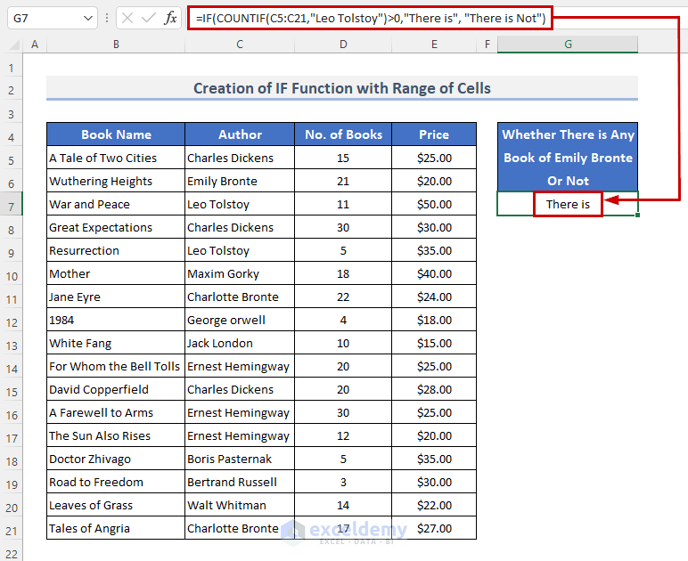
We’ll check whether there is any book by the author Emily Bronte.
STEPS:
- Select a cell and enter this formula into that cell.
=IF(COUNTIF(C5:C21,"Emily Bronte")>0,"There is", "There is Not")- Press Enter to see the result.
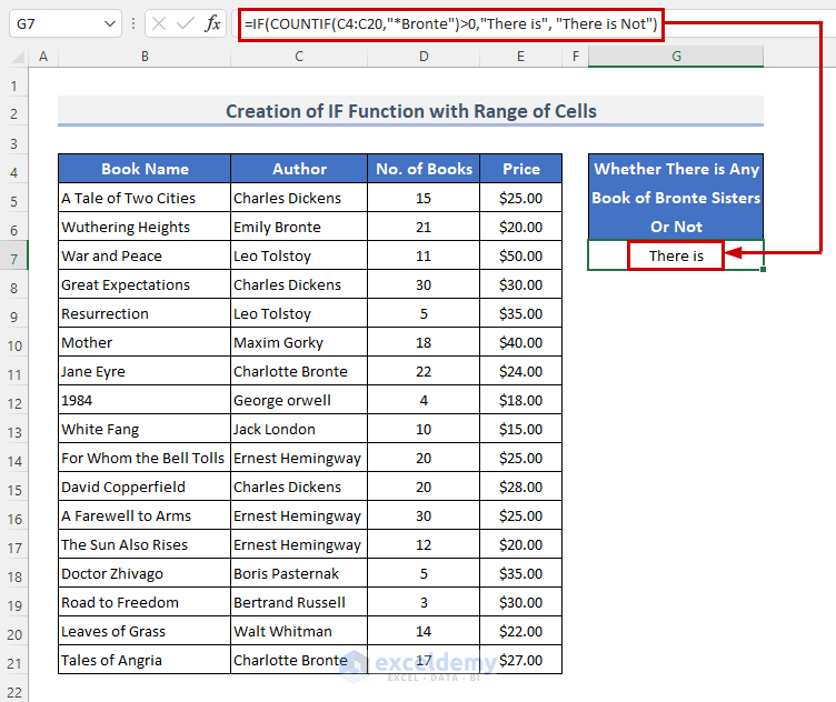
- If you want an approximate match, you can use Wildcard Characters (*,?,~) within the COUNTIF function. To find out whether there is any book by the Bronte sisters (Both Emily Bronte and Charlotte Bronte), use the following formula:
=IF(COUNTIF(C4:C20,"*Bronte")>0,"There is", "There is Not")- Hit the Enter key to show the outcome.
How Does the Formula Work?
- COUNTIF(C5:C21,”Emily Bronte”) returns the number of times the name “Emily Bronte” appears in the range C5:C21.
- COUNTIF(C5:C21,”Emily Bronte”)>0 returns TRUE if the name appears at least once in the range, and returns FALSE if the name doesn’t appear.
- IF(COUNTIF(C5:C21,”Emily Bronte”)>0,”There is”, “There is Not”) returns “There is” if the name appears at least once, and returns “There is Not” if the name does not appear.
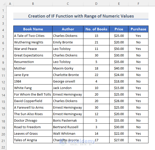
Example 2 – IF Function with a Range of Numeric Values in Excel
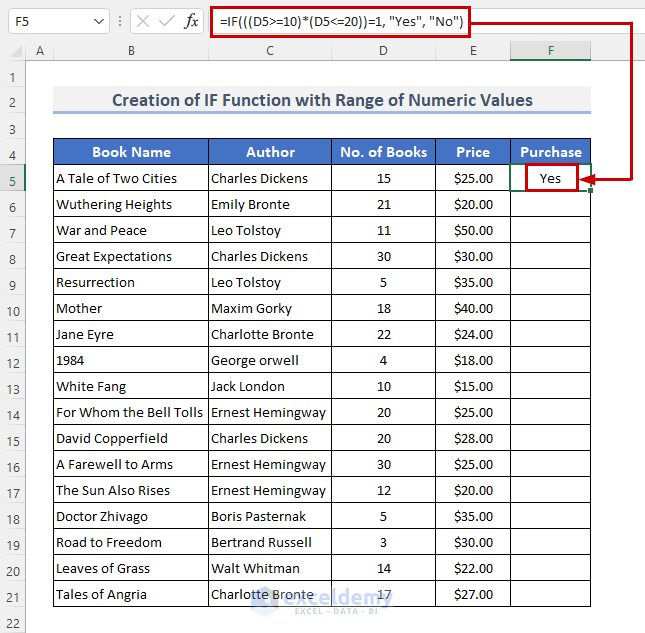
We will create a list of values from a range that falls between two given numbers. Let’s check if their prices fall between $10 and $20.
Steps:
- Select the cell where you want to see the result.
- Enter the formula there.
=IF(((D5>=10)*(D5<=20))=1, "Yes", "No")- Press Enter.
- Drag the Fill Handle icon down to duplicate the formula over the range or double-click on the plus (+) symbol.
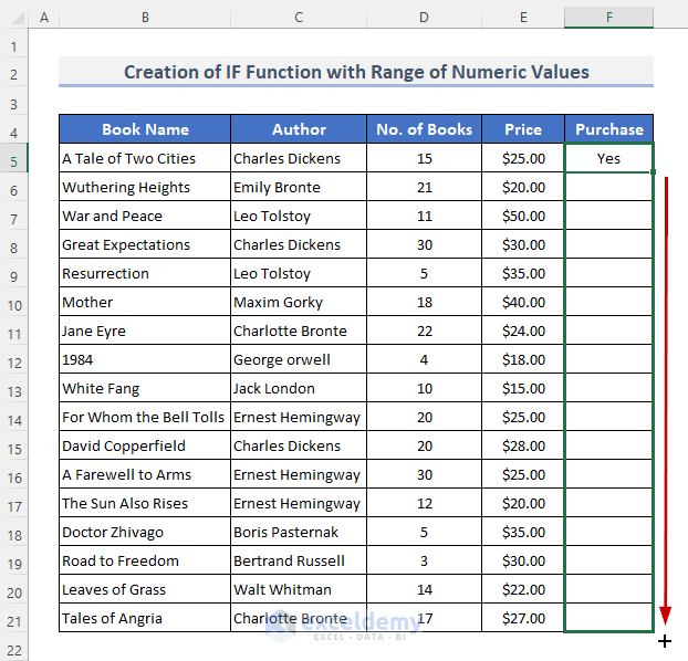
- Here’s the result.
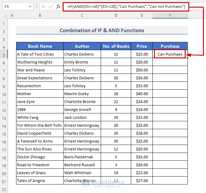
Example 3 – Applying AND Conditions with the IF Function for a Range of Values
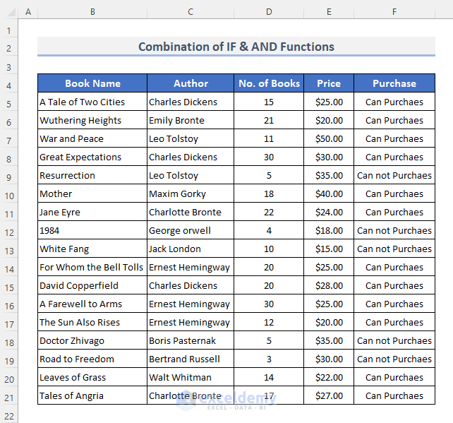
Let’s check two conditions: the number of books is greater than 10 and the price of the book is greater than 20.
Steps:
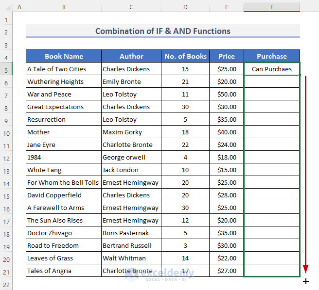
- Select a cell F5 and enter the formula:
=IF(AND(D5>=10,E5>=20),"Can Purchase","Can not Purchase")- Press the Enter key.
- Alternatively, use the following formula:
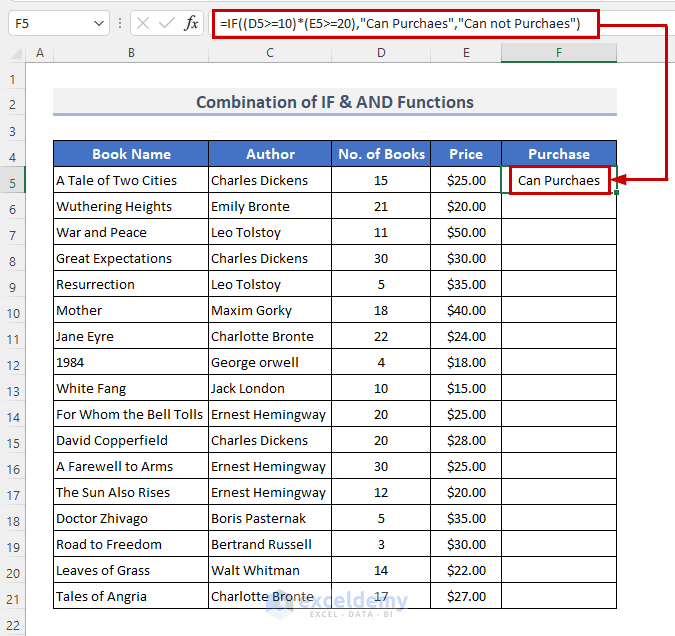
- Drag the Fill Handle symbol down or double-click it to AutoFill the range.
- Here’s the result.
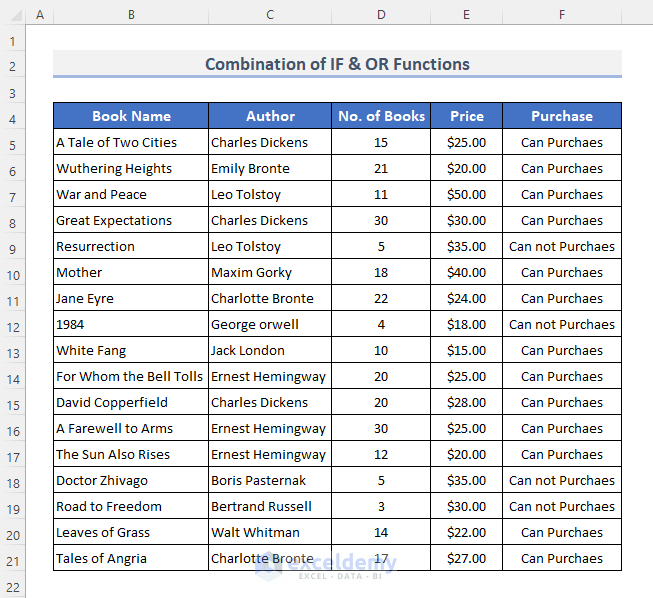
Example 4 – Using the IF Function with OR Conditions for a Range of Values
Steps:
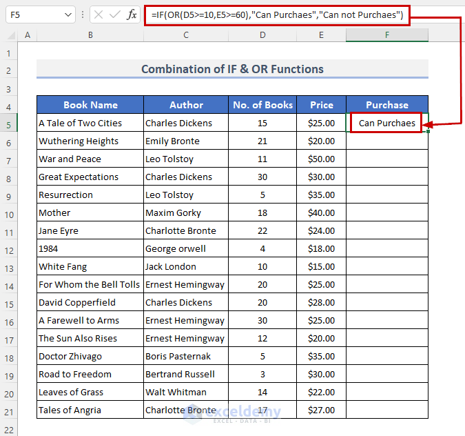
- Select the first cell where we want to see the result.
- Insert the formula.
=IF(OR(D5>=10,E5>=60),"Can Purchase","Can not Purchase")- Press the Enter key.
- Alternatively, use the following formula:
=IF((D5>=10)+(E5>=60),"Can Purchase","Can not Purchase")- Hit Enter to see the result.

- Drag the Fill Handle icon to copy the formula over the range or double-click the Fill Handle.
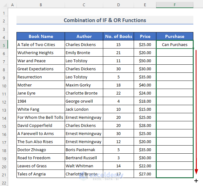
- Here’s the result.
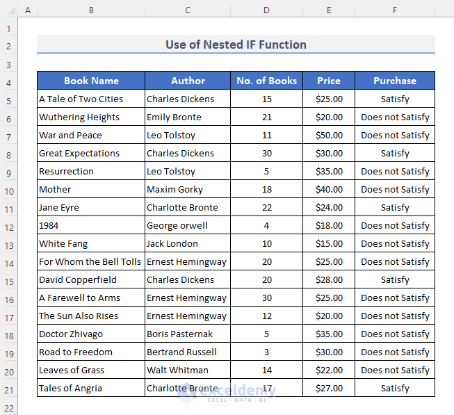
Example 5 – Using a Nested IF Function for a Range of Values in Excel
We’ll check whether the price is higher than $30, then check if the number of books is higher than 15. After that, we’ll check if the author’s name starts with the letter C. If all of these apply, we’ll return “Satisfy“. Otherwise, we’ll return “Does not Satisfy“.
Steps:
- Select the first result cell and insert the following formula:
=IF(E5>=20,IF(D5>=15,IF(LEFT(C5,1)="C","Satisfy","Does not Satisfy"),"Does not Satisfy"),"Does not Satisfy")- Hit the Enter key to see the outcome.
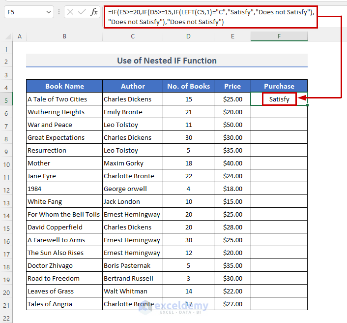
- Drag the Fill Handle icon down to duplicate the formula over the range.
Read More: How to Use IF Function with Multiple Conditions in Excel
Example 6 – Combining IF and SUM Functions in Excel for a Range of Values
Steps
- Select G6 and put the following formula into it:
=IF(SUM(D5:D21)>=80, "Good", IF(SUM(D5:D21)>=50, "Satisfactory", "Poor"))- Press the Enter key to see the outcome.
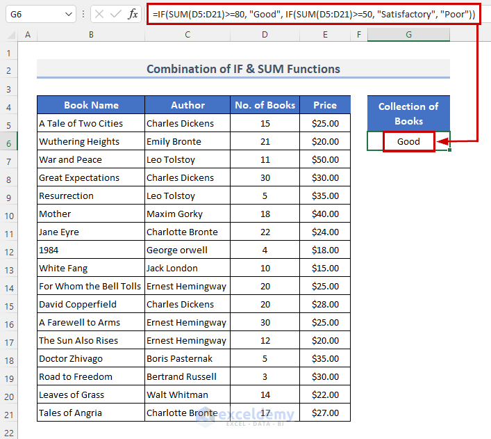
How Does the Formula Work?
- SUM(D5:D21) this part adds the values of the range and returns the total number of books as a result.
- SUM(D5:D21)>=80 and SUM(D5:D21)>=50 checks whether the condition is met.
- IF(SUM(D5:D21)>=80, “Good”, IF(SUM(D5:D21)>=50, “Satisfactory”, “Poor”)) reports the result. In our case, the result was “Good”.
Example 7 – Joining IF and AVERAGE Functions for a Range of Values
Steps:
- Use the following formula in G6:
=IF(AVERAGE(D5:D21)>=20, "Good", IF(AVERAGE(D5:D21)>=10, "Satisfactory", "Poor"))- Hit Enter.
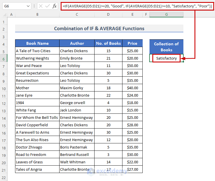
How Does the Formula Work?
- AVERAGE(D5:D21) calculates the average number of books.
- AVERAGE(D5:D21)>=20 and AVERAGE(D5:D21)>=10 verify whether the condition was satisfied.
- IF(AVERAGE(D5:D21)>=20, “Good”, IF(AVERAGE(D5:D21)>=10, “Satisfactory”, “Poor”)) reveals the outcome. The outcome in our situation is “Satisfactory”.
Example 8 – Using IF and EXACT Functions to Match a Range of Values in Excel
Steps:
- Insert the following formula in the result cell.
=IF(EXACT($C$5:$C$21,"Leo Tolstoy"), "Yes", "No")- Hit Enter (use Ctrl + Shift + Enter for Excel versions other than Excel 365).
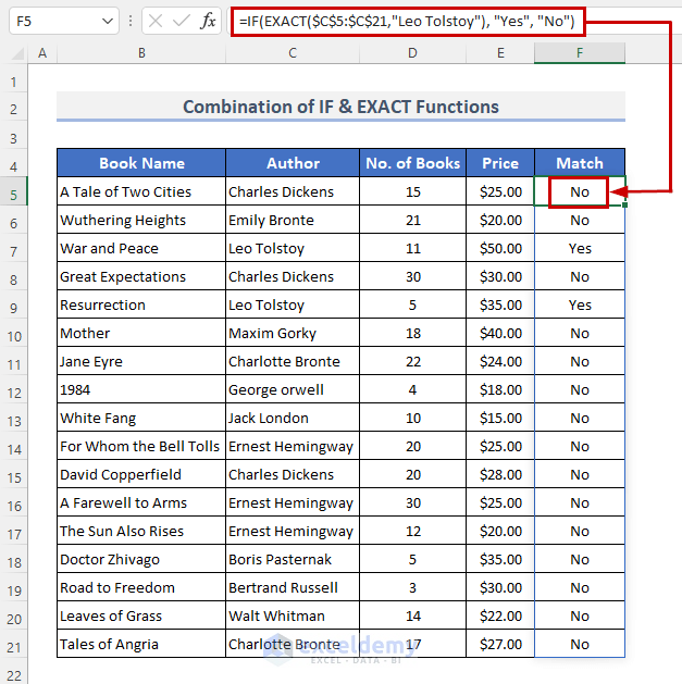
How Does the Formula Work?
- EXACT($C$5:$C$21,”Leo Tolstoy”) shows whether both data are an exact match or not.
- IF(EXACT($C$5:$C$21,”Leo Tolstoy”), “Yes”, “No”) check the logic and return the result.
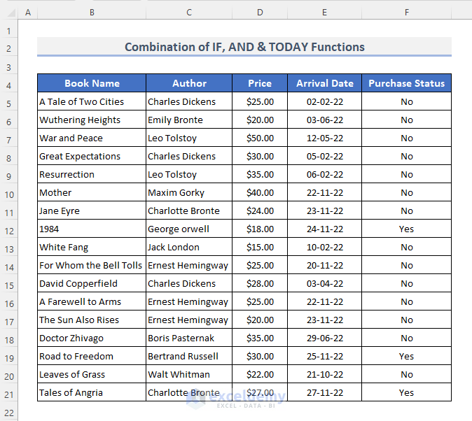
Example 9 – Combining IF, AND, and TODAY Functions to Get a Date in Excel
We want to check whether the arrival date is within 7 days.
Steps:
- Use the following formula:
=IF(AND(E5>TODAY(), E5<=TODAY()+7), "Yes", "No")- Press Enter.
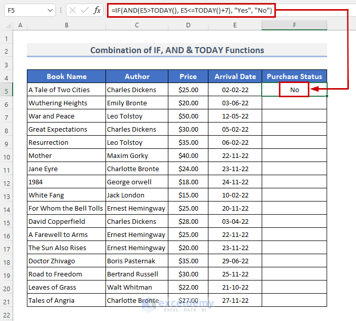
- Copy the formula over the result range with the Fill Handle.
Example 10 – Obtaining Highest or Lowest Value by Combining IF, MAX, and MIN Functions
Steps:
- Select the cell where we want to put the result.
- Insert the following formula into that cell.
=IF(D5=MAX($D$5:$D$21), "Good", IF(D5=MIN($D$5:$D$21), "Not Good", " Average"))- Press Enter.

How Does the Formula Work?
- MAX($D$5:$D$21) returns the maximum value of the range.
- MIN($D$5:$D$21) returns the minimum value of the range.
- IF(D5=MAX($D$5:$D$21), “Good”, IF(D5=MIN($D$5:$D$21), “Not Good”, ” Average”)) shows the result after comparison.
Things to Remember
- If you’re attempting to divide a number by zero in your formula, you may see #DIV/0! error.
- The #VALUE! error occurs when you enter the incorrect data type into the calculation.
- If we relocate the formula cell or the reference cells, the #REF! the error will appear.
- The #NAME! error will show you misspell the name of a function in your formula.
Download the Practice Workbook
Related Articles
<< Go Back to Excel IF Function | Excel Functions | Learn Excel
Get FREE Advanced Excel Exercises with Solutions!
