How to Use MAX IF Function in Excel (4 Practical Examples)

What Is MAX-IF Formula in Excel?

MAX Function

The MAX function is one of the most commonly used functions in Excel. It returns the maximum value from a selected range. The MAX function ignores the logical values and text. The syntax of the MAX function is given below.

MAX (number1, [number2], ...)

IF Function

The IF function is another essential function of Excel. The IF function returns a specified value, if a given logical test is satisfied. The syntax for the IF function is given here.

=IF(logical_test, [value_if_true], [value_if_false])

We will use the combination of the MAX function and the IF function. In general, the MAX IF formula returns the largest numeric value that satisfies one or more criteria in a given range of numbers, dates, texts, and other conditions. After combining these two functions, we get a generic formula like this.

=MAX(IF(criteria_range=criteria, max_range))

Example 1 – Using Excel MAX-IF Function with an Array Formula

Case 1.1 – Inserting a MAX-IF Formula with Single Criterion

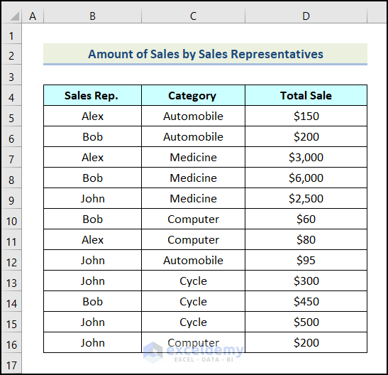
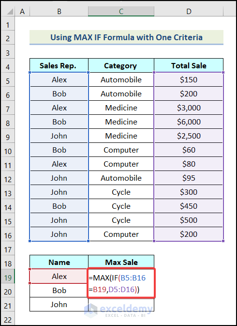
We need to find the maximum number of sales of the Sales Rep.

Steps:

Create a table anywhere in the worksheet, and in the name column, insert the names of the Sale Reps.

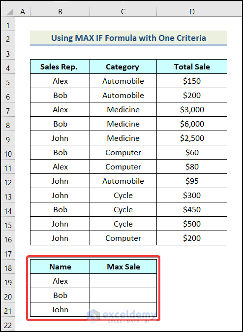
Apply the MAX IF formula:

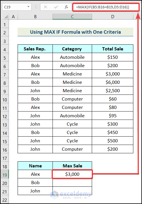
=MAX(IF(B5:B16=B19,D5:D16))

The range of cells B5:B16 indicates the cells of the Sales Rep. column, cell B19 refers to the selected Sales Rep, and the range of cells D5:D16 represents the cells of the Total Sale column.

Formula Breakdown

max_range is the Total Sale column (D5:D16).
criteria is the name of the Sales Rep (B19).
criteria_range Is the Sales Rep. column (B5:B16).
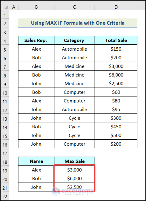
Output → $3,000.

Since this is an array formula, press Shift + Ctrl + Enter.

For the other two names, we will use the same formula.

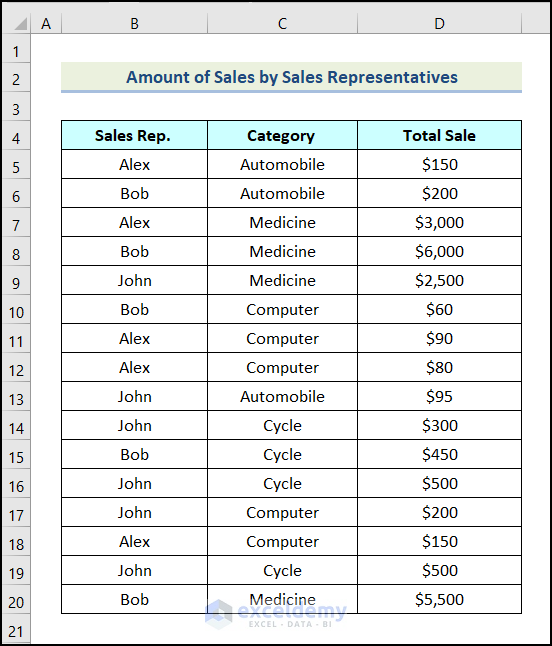
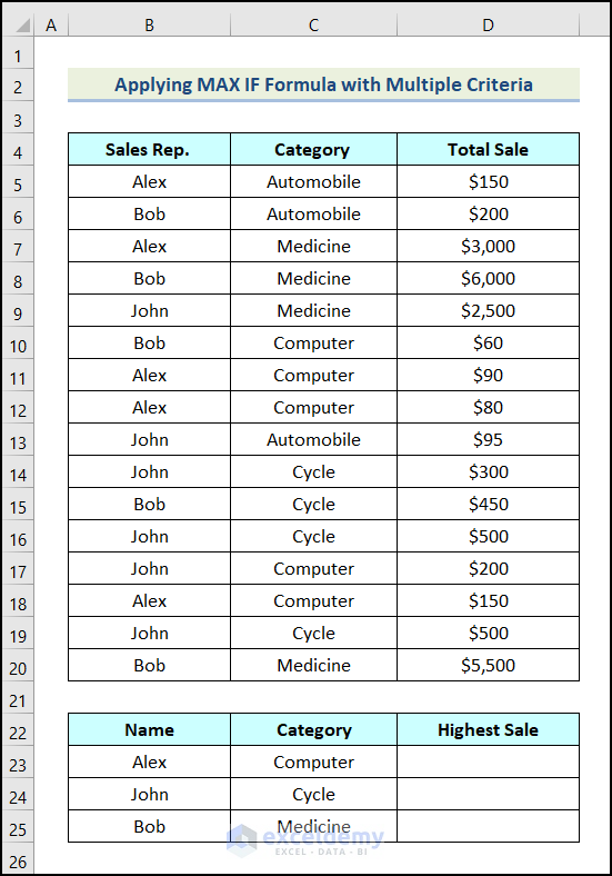
Case 1.2 – Applying a MAX-IF Formula with Multiple Criteria

We have more than one Sales Rep named “Alex”, “Bob”, and “John” in the Computer, Cycle, and Medicine category. We have to find the highest number of sales made by these Sales Reps in each category.

Steps:

Create a table anywhere in the worksheet and the name and the Category column insert the given criteria.

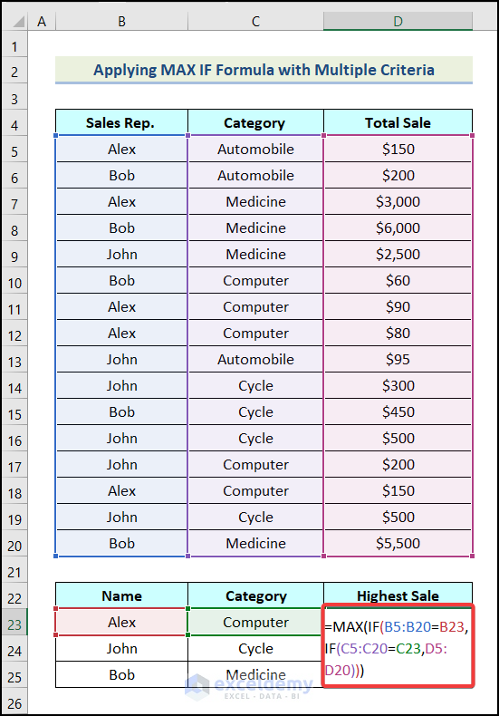
Apply the MAX IF formula:

=MAX(IF(B5:B20=B23,IF(C5:C20=C23,D5:D20)))

Here, range of cells C5:C20 indicates the cells of the Category column, cell C23 refers to the selected category.

Formula Breakdown

In the first IF function,
- C5:C20=C23 → It is the logical_test argument.
- D5:D20 → This indicates the [value_if_true] argument.
- Output → {FALSE;FALSE;FALSE;FALSE;FALSE;60;90;80;FALSE;FALSE;FALSE;FALSE;200;150;FALSE;FALSE}.
In the 2nd IF function,
- B5:B20=B23 → This is the logical_test argument.
- IF(C5:C20=C23,D5:D20) → It refers to the [value_if_true] argument.
- Output → {FALSE;FALSE;FALSE;FALSE;FALSE;FALSE;90;80;FALSE;FALSE;FALSE;FALSE;FALSE;150;FALSE;FALSE}
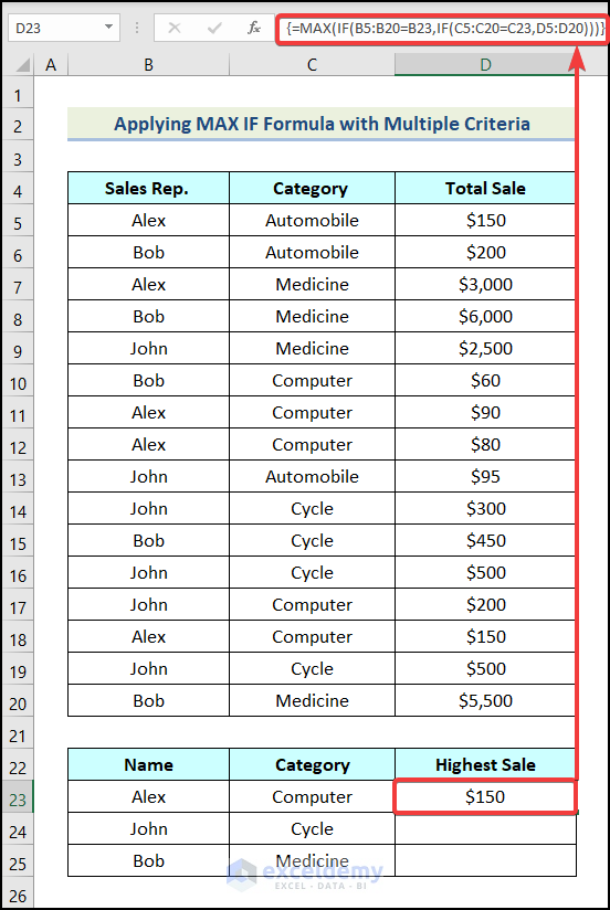
The MAX function returns the maximum value from the array.
- Output → $150.

Press Shift + Ctrl + Enter simultaneously to apply the formula.

We have found our maximum number.

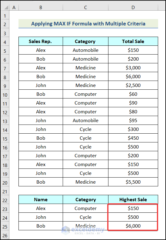
Apply the same formula to the other cells.

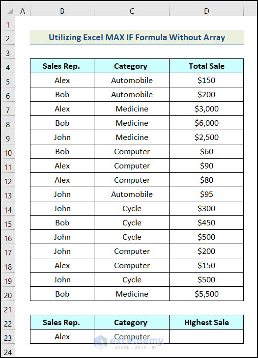
Example 2 – Inserting the Excel MAX-IF Function Without an Array

Steps:

Our goal is to find as many sales as possible for ““Alex”” in the “Computer” category.

Create a table as shown in the following picture.

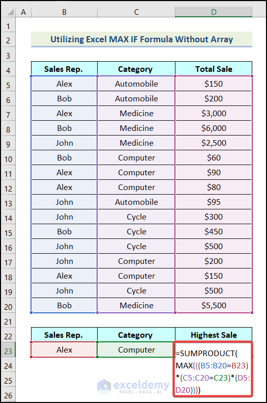
Apply the formula given below in cell D23.

=SUMPRODUCT(MAX(((B5:B20=B23)*(C5:C20=C23)*(D5:D20))))

Formula Breakdown

max_range denotes the Total Sale column (D5:D20)
Criteria2 is the name of the Category (C23)
criteria_range2 refers to the Category column (C5:C20)
Criteria1 is the name of the Sales Rep (B23)
criteria_range1 indicates the Sales Rep Column (B5:B20)
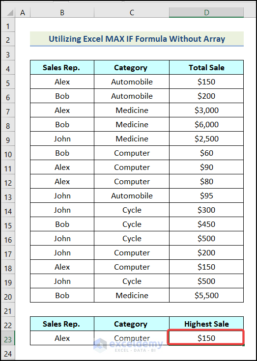
Output → $150.

Press Enter and the maximum value will be available in cell D23 as demonstrated in the image below.

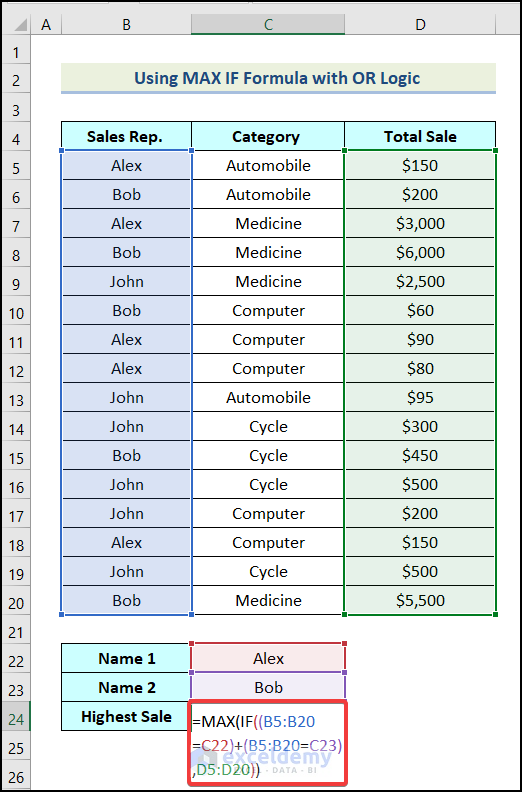
Example 3 – Combining a MAX-IF Formula with OR Logic

Steps:

Insert a new table as shown in the following image.

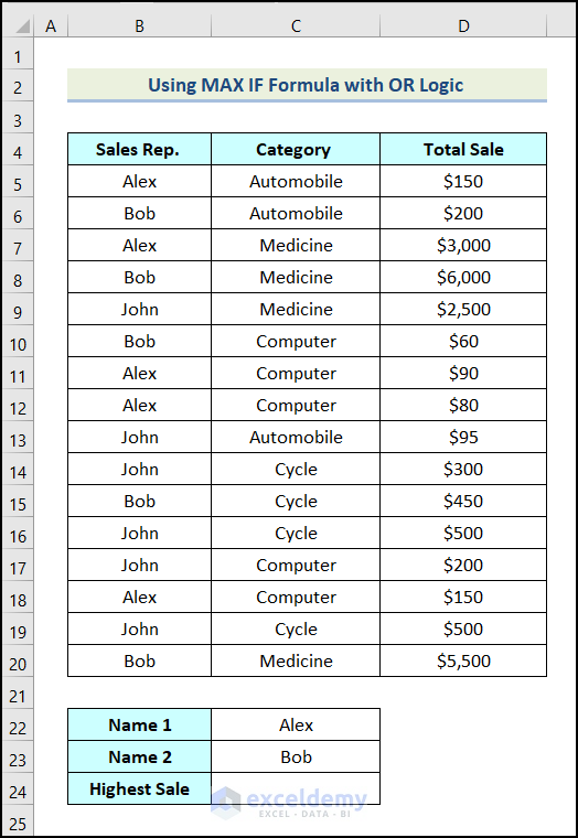
Use the following formula in cell C24.

=MAX(IF((B5:B20=C22)+(B5:B20=C23),D5:D20))

Cell C22 refers to the first selected name, and cell C23 indicates the second selected name.

Formula Breakdown

max_range is the Total Sale column (D5:D20).
criteria2 is the name of the Category (C23).
criteria_range2 refers to the Category column (B5:B20).
criteria1 is the name of the Sales Rep (C22).
criteria_range1 indicates the Sales Rep Column (B5:B20).

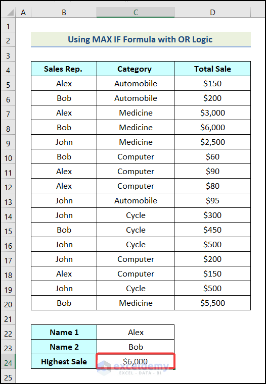
Apply the formula by pressing Shift + Ctrl + Enter.

We will get the maximum sales amount between “Alex” and “Bob” in cell C24.

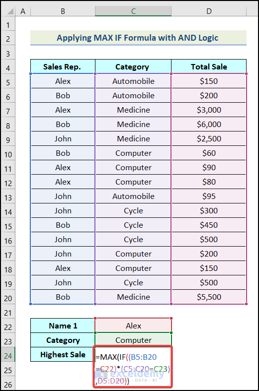
Example 4 – Applying the MAX-IF Formula with AND Logic

Steps:

Create a new table as shown in the following image.

Use the following formula in cell C24.

=MAX(IF((B5:B20=C22)*(C5:C20=C23),D5:D20))

Formula Breakdown

max_range represents the Total Sale column (D5:D20).
criteria2 refers to the name of the Category (C23).
criteria_range2 indicates the Category column (B5:B20).
criteria1 is the name of the Sales Rep (C22).
criteria_range1 is the Sales Rep Column (B5:B20).

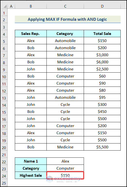
Hit Enter.

You will get the following output on your worksheet as demonstrated in the image below.

How to Use the MAXIFS Function in Excel

The MAXIFS function is available from Excel 2019 onward.

Steps:

Insert a table and input your criteria as demonstrated in the following image.

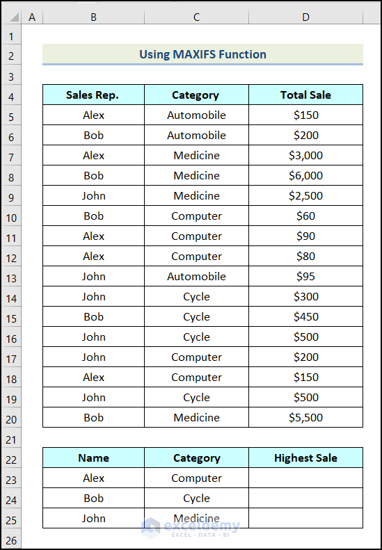
We need to find the maximum sales for “Alex”, “Bob”, and “John” in a given category.

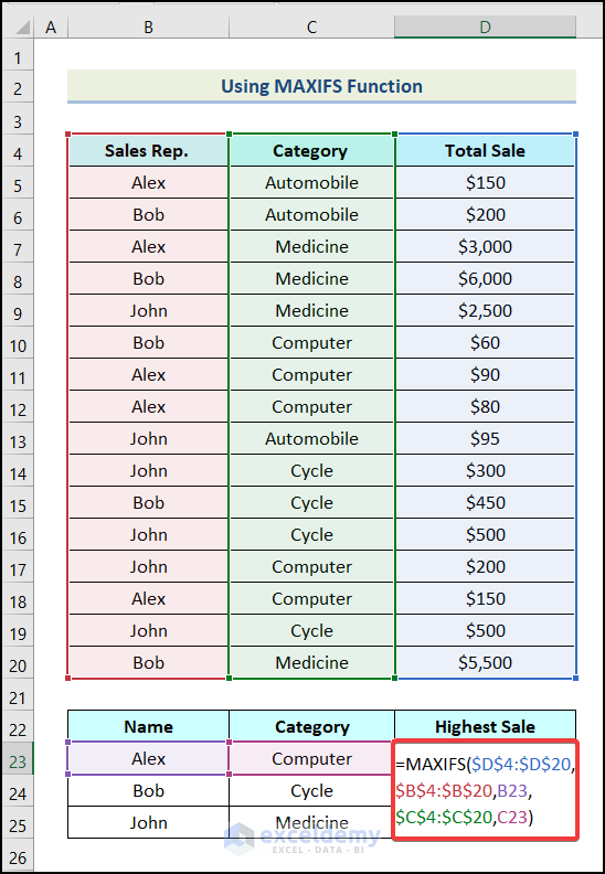
Use the formula given below in cell D22.

=MAXIFS($D$4:$D$20,$B$4:$B$20,B23,$C$4:$C$20,C23)

Formula Breakdown

max_range is the Total Sale column ($D$4:$D$20).
criteria_range1 is the Sales Rep. column ($B$4:$B$20).
criteria1 Is the name of the Sales Rep (B23).
criteria_range2 is the name of the Category column ($C$4:$C$20).
criteria2 is the name of the Category (C23).
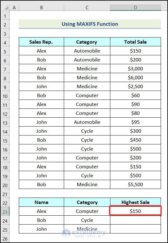
Output → $150.

Press Enter and you will get the following output on your worksheet.

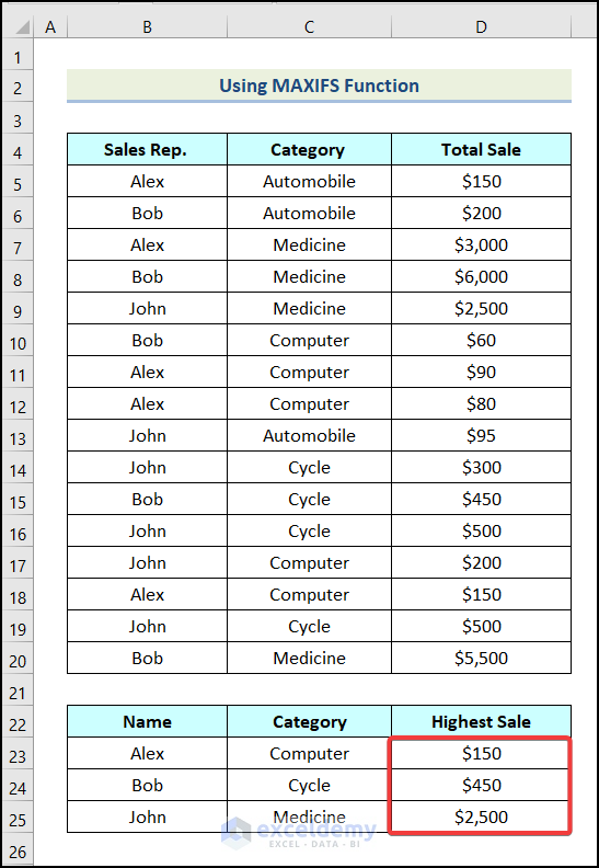
Use the AutoFill option of Excel to get the remaining outputs.

Things to Remember

The MAX-IF is an Array Formula so in the older versions of Excel, you have to press Shift + Ctrl + Enter simultaneously to apply it.
The MAXIFS function is only available for Excel 2019 onward and Office 365.

Download the Practice Workbook

Using MAX IF Function.xlsx