How to Check If a Value Lies Between Two Numbers and Return a Result in Excel

Understanding the IF-THEN Formula

In a nutshell, Excel’s IF-THEN formula allows you to create conditional logic within a worksheet. It checks whether a specified condition is true or false and performs a specific task based on that condition.

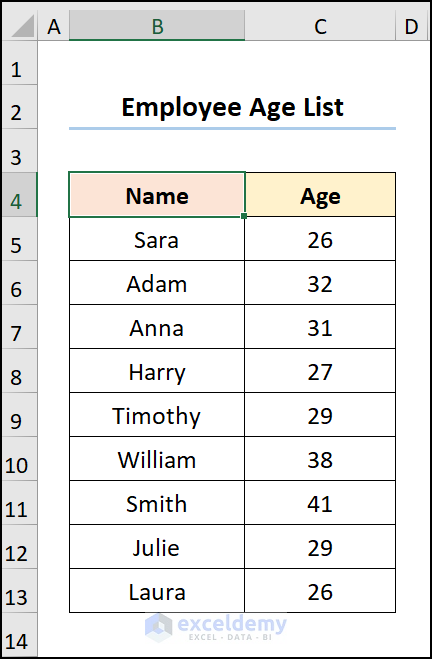
Scenario – Employee Age List Dataset

Suppose we have an Employee Age List dataset with employees’ names and their corresponding ages in cells B4:C13.

Method 1 – Using the Excel AND Function

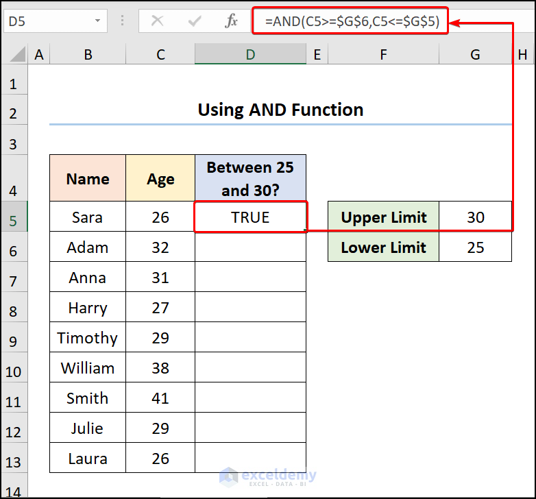
Let’s start with the simplest approach: using the AND function to check if an employee’s age falls between 25 and 30 years. Follow these steps:

Go to cell D5.
Enter the following formula:

=AND(C5>=$G$6,C5<=$G$5)

Here:

C5 represents the employee’s age.
$G$6 is the upper limit (30 years).
$G$5 is the lower limit (25 years).

Note: Use absolute cell references by pressing the F4 key on your keyboard.

Formula Breakdown:

The formula AND(C5>=$G$6, C5<=$G$5) checks whether both arguments are TRUE. If they are, it returns TRUE. Specifically:

C5>=$G$6 is the logical1 argument.
C5<=$G$5 is the logical2 argument.

Since both arguments evaluate to TRUE, the function returns the output TRUE.

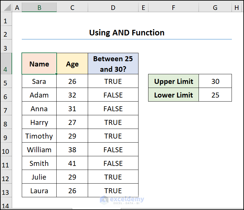
Use the Fill Handle tool to copy the formula down to other cells.

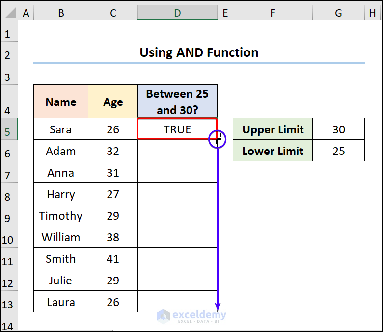
Your result should resemble the image below:

Method 2 – Using IF and AND Functions to Determine If a Value Lies Between Two Numbers and Return Text

Select cell D5.
Enter the following formula:

=IF(AND(C5>=$G$6,C5<=$G$5),"Yes","No")

In this formula:

C5 represents the employee’s age.
$G$6 is the upper limit (30 years).
$G$5 is the lower limit (25 years).

Formula Breakdown:

- AND(C5>=$G$6, C5<=$G$5) checks whether both arguments are TRUE. If they are, it returns TRUE.
- The entire formula evaluates whether the age in cell C5 falls between the upper and lower limits.
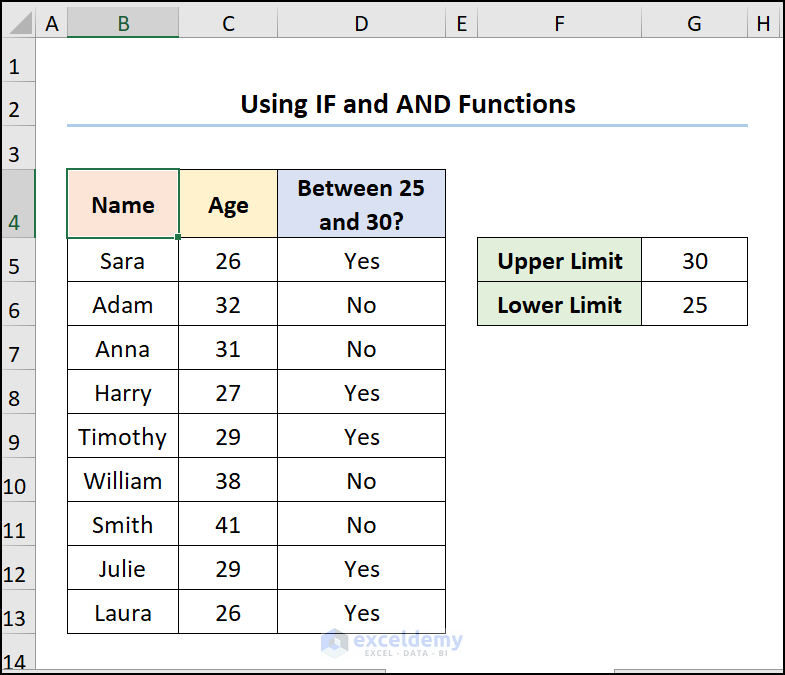
- If TRUE, it returns “Yes”; otherwise, it returns “No.”

The output will be either “Yes” or “No.”

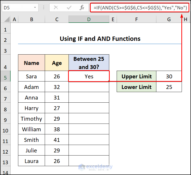
Your result should resemble the image below:

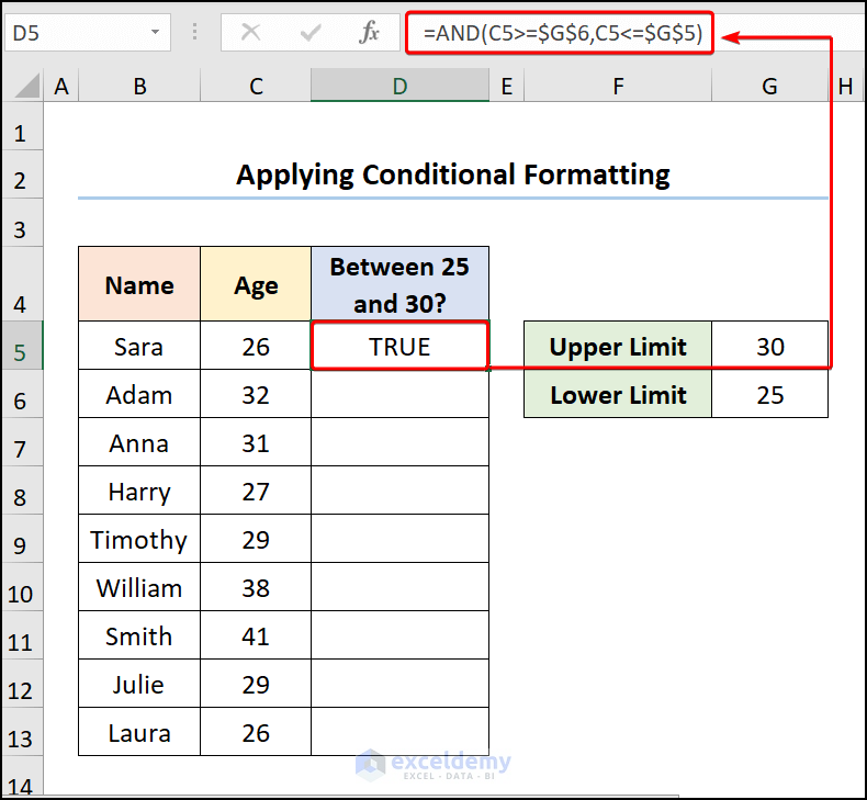
Method 3 – Applying Excel Conditional Formatting

Another approach involves using Conditional Formatting to highlight cells where a value lies between two numbers. Here’s how:

Go to cell D5 and enter the formula:

=AND(C5>=$G$6,C5<=$G$5)

Again, C5, $G$6, and $G$5 represent the age, upper limit, and lower limit, respectively.

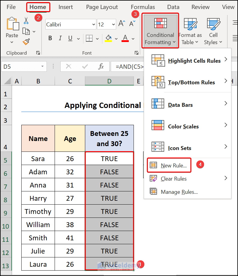
Select the range of cells D5:D13.
Under the Home tab, click the Conditional Formatting drop-down and choose New Rule.

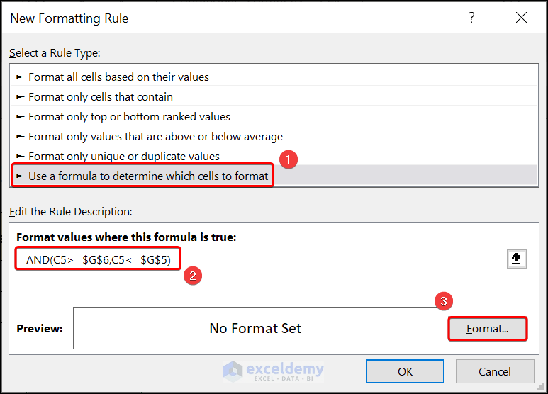
In the New Formatting Rule wizard, select Use a formula to determine which cells to format.
Enter the same formula:

=AND(C5>=$G$6,C5<=$G$5)

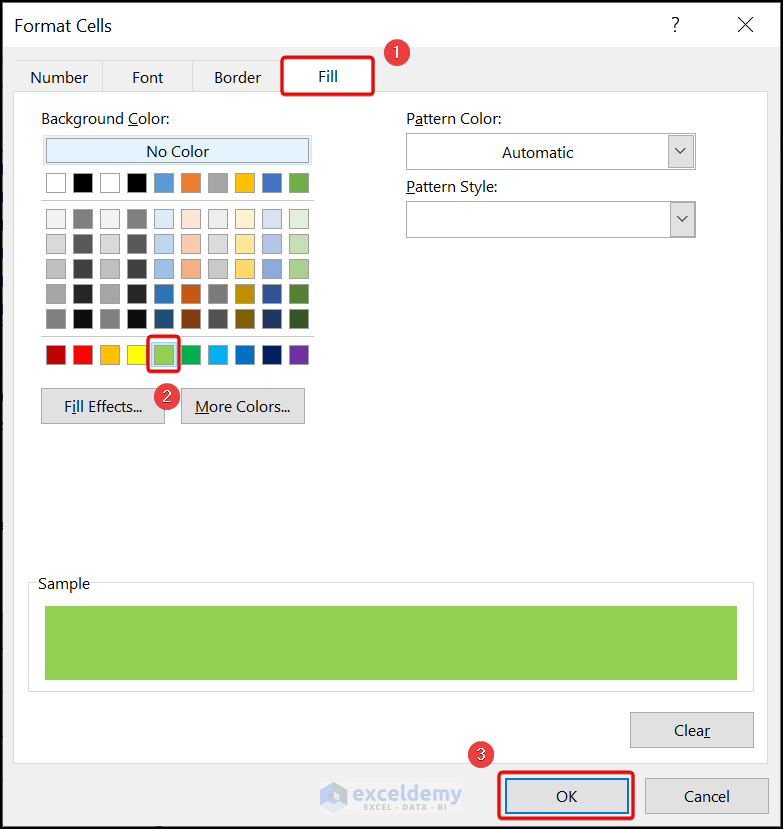
Click the Format box to specify the cell color.

In the Format Cells wizard, go to the Fill tab and choose a color (e.g., Light Green).
Click OK.

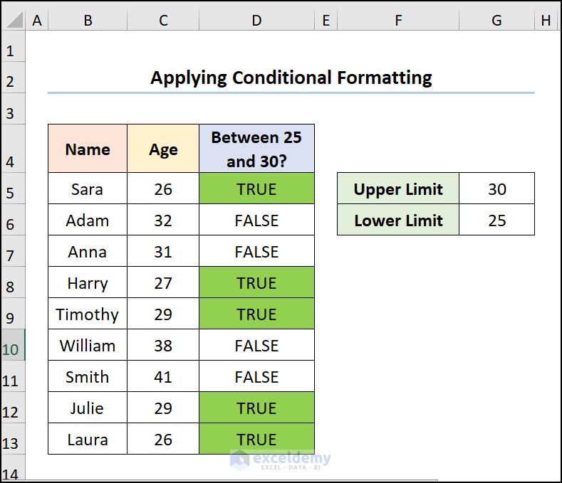
The result will highlight cells where the age falls within the specified limits.

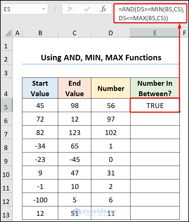
Method 4 – Returning TRUE/FALSE If a Value Lies Between Two Numbers Using Excel AND, MIN, and MAX Functions

Here, we’ll combine the AND, MIN, and MAX functions to check if a third number lies between these two numbers.
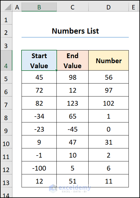
Let’s consider the Numbers List dataset in the B4:D13 cells. Here, the dataset shows a Start Value, End Value, and Number respectively.

Go to cell E5.
Enter the following formula:

=AND(D5>=MIN(B5,C5),D5<=MAX(B5,C5))

In this formula:

B5, C5, and D5 represent the start value, end value, and the number, respectively.

Formula Breakdown:

AND(D5>=MIN(B5,C5), D5<=MAX(B5,C5)) checks whether both arguments are TRUE. If they are, it returns TRUE.
The logical1 argument (D5>=MIN(B5,C5)) checks if the value in cell D5 is greater than or equal to the larger of the two values in cells B5 and C5.
The logical2 argument (D5<=MAX(B5,C5)) checks if the value in cell D5 is less than or equal to the smaller of the two values in cells B5 and C5.
If both arguments evaluate to TRUE, the function returns TRUE.

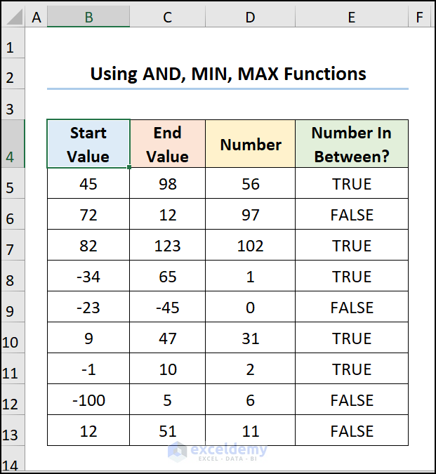
- The output will be either TRUE or FALSE.

Your result should resemble the image below:

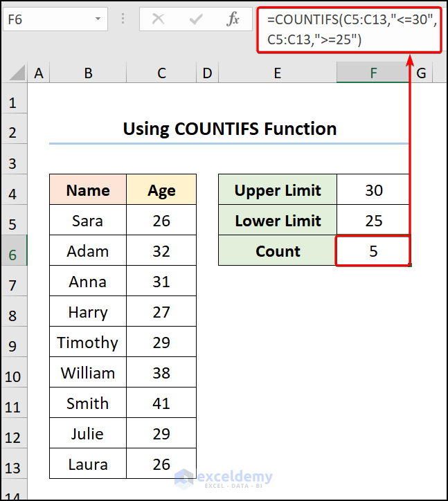
Using the COUNTIFS Function to Count Between Two Numbers in Excel

If you want to count the number of occurrences between two numbers, you can use the COUNTIFS function. Let’s see it in action:

Navigate to cell F6.
Enter the following formula:

=COUNTIFS(C5:C13,"<=30",C5:C13,">=25")

Here:

C5:C13 represents the range of cells containing employees’ ages.
30 and 25 are the upper and lower limits, respectively.

Formula Breakdown:

COUNTIFS(C5:C13, “<=30”, C5:C13, “>=25”) counts the number of cells that meet specific conditions.
The first set of criteria (<=30) counts all age values that are less than or equal to 30.
The second set of criteria (>=25) counts values that are greater than or equal to 25.
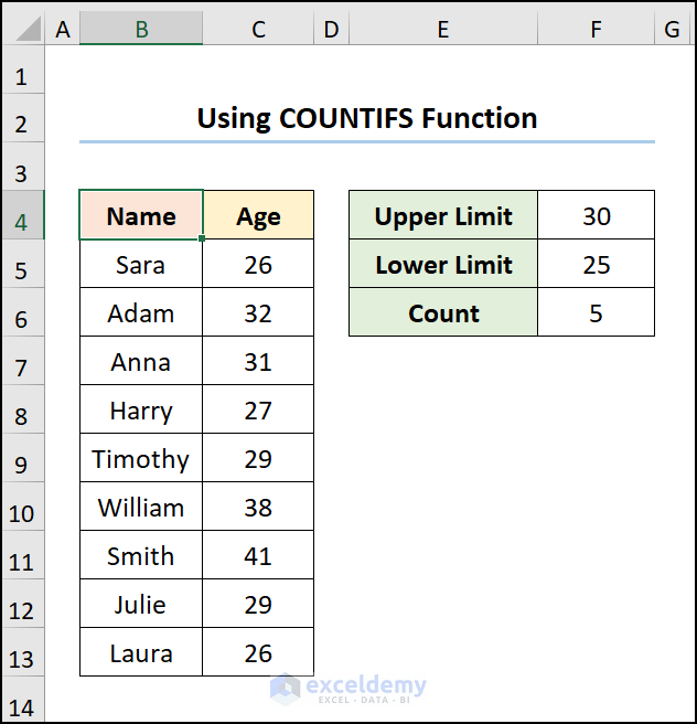
The result shows the number of ages between 25 and 30.