How to Make Yes 1 and No 0 in Excel (2 Effective Methods)

Method 1 – Make Yes 1 and No 0 Using IF Function in Excel

Steps:

• Click on cell D5.
• Enter the following formula and press Enter.

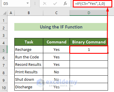
• You will get 1 as the command is yes for the first task.
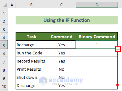
• Drag the Fill Handle to copy the formula for all the cells below.

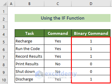
Making all yes into 1 and all no into 0 in Excel will give the output as shown in the image below.

Method 2 – Use Find & Replace Option

Steps:

• Select cells C5 to C10 and Copy.

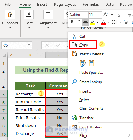
• Select cell D5 and Paste.

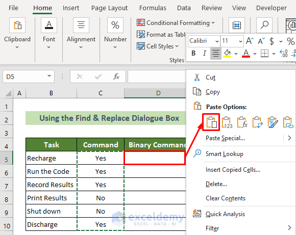
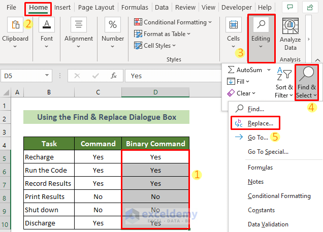
• Select all the pasted cells from D5 to D10.
• Go to the Home tab >> Editing group >> Find & Select tool >> Replace.

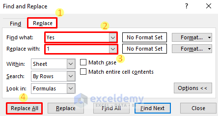
• The Find and Replace window will appear.
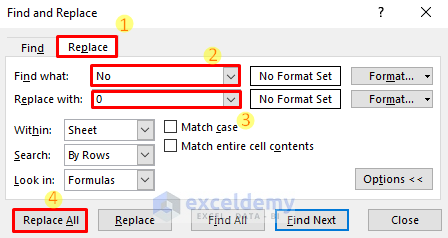
• Go to the Replace tab.
• Enter Yes in the Find what: text box and insert 1 in the Replace with: text box.
• Click on the Replace All button.

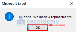
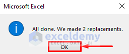
• A Microsoft Excel confirmation window will appear. Click OK.

• In the Replace tab, enter No in the Find what: text box and enter 0 in the Replace with: text box.
• Click on Replace All.

• A Microsoft Excel confirmation window will appear. Click OK.

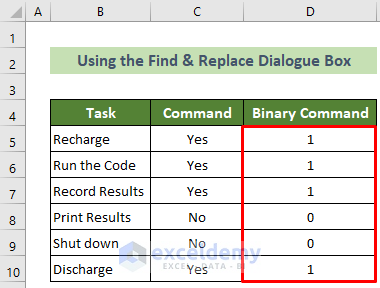
It will make 1 as yes and 0 as No in Excel as shown in the image below.

Read More: [Fixed!] IF Function Is Not Working in Excel

How to Make 1 as Yes and 0 as No in Excel?

Steps:

• You are given 1 and 0 as commands. You need to have them as Yes and No.
• Select C5:C10 cells and Copy.

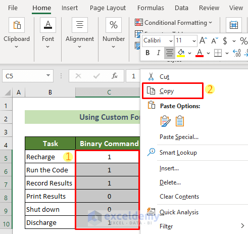
• Select the D5 cell and Paste.

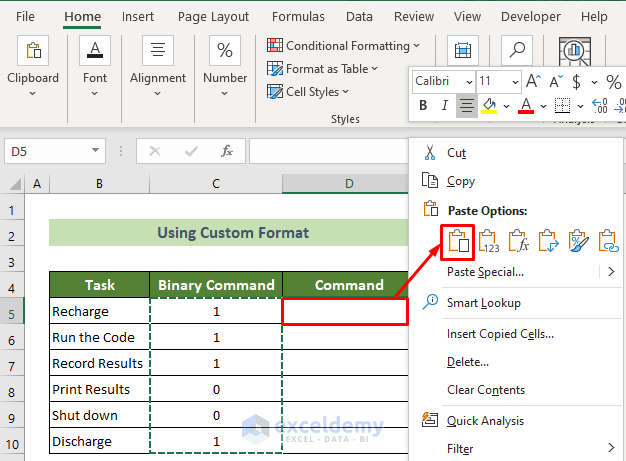
• Select the cells D5:D10 and right-click to get the Format Cells option.

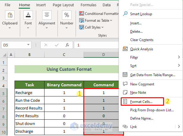
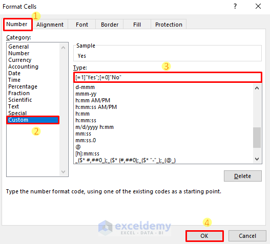
• The Format Cells window will appear.
• Go to the Number tab >> choose the Custom option from the Category: pane >> enter any of the following formats in the Type: text box.

Or,

• Click OK.

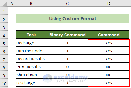
All the 1 and 0 will have Yes and No output.

Download Practice Workbook

Related Articles

<< Go Back to Excel IF Function | Excel Functions | Learn Excel