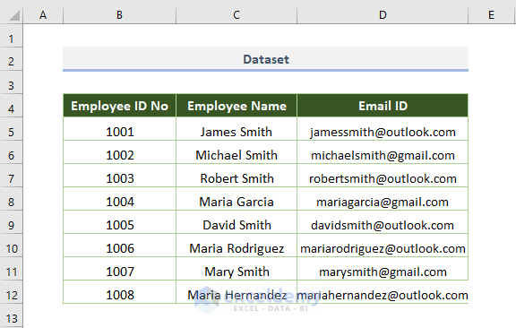
Below is a dataset where employee names are provided with their Employee ID No and Email ID.
Method 1 – Applying the LOOKUP Function to Extract Text
The function returns the value in a single row or column from a similar position in the row or column.
If the lookup value is 1003 (Employee ID) and you need to find the employee name for the ID, use the following formula:
=LOOKUP(F5,B5:B12,C5:C12) F5 is the lookup value, B5:B12 is Employee ID’s lookup vector (cell range), and C5:C12 is Employee Name’s result vector (cell range).
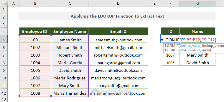
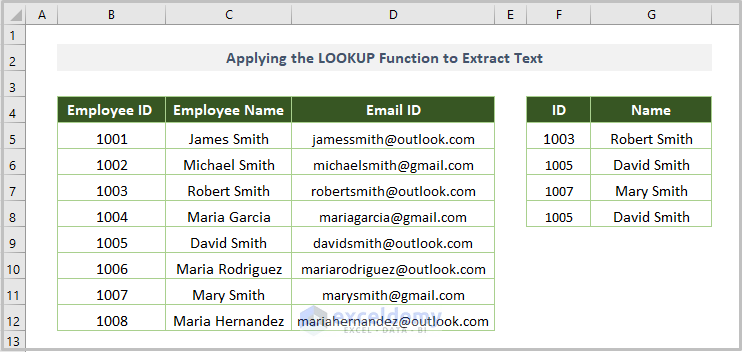
You’ll get the following output where the names of employees are available based on the ID.
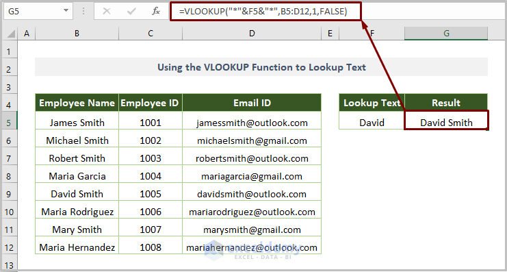
Method 2 – Using the VLOOKUP Function to Lookup Text
The function is used to extract the text for a certain cell.
The adjusted formula with wildcards for finding text value is:
=VLOOKUP("*"&F5&"*",B5:D12,1,FALSE)F5 is the lookup text, B5:D12 is the table array (dataset from which to retrieve the text), 1 is the column index number, and FALSE is the exact matching.
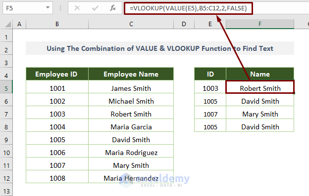
Method 3 – Combining the VALUE & VLOOKUP Functions to Find Text
The VALUE function returns the number from a looking text value. We can utilize this function along with the VLOOKUP function to find the text.
The combined formula will be like the following:
=VLOOKUP(VALUE(F5),B5:C12,2,FALSE)F5 is the lookup text, B5:D12 is the table array (dataset from which to retrieve the text), 2 is the column index number, and FALSE is for the exact matching.
VALUE(F5) returns the number, and then the VLOOKUP extracts the text value.
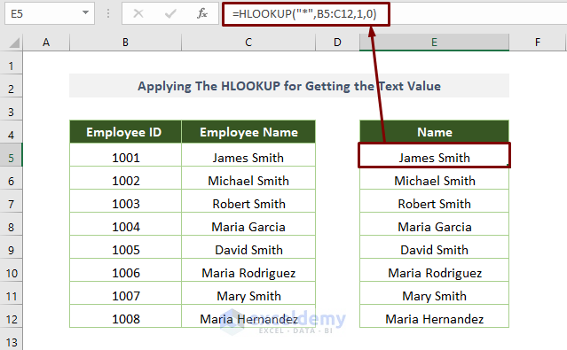
Method 4 – Utilizing HLOOKUP to Get the Text Value
The HLOOKUP function returns a value based on the lookup value in a row (horizontal lookup).
We can utilize the function to get the text value sequentially using Asterisk (*) at the beginning of the formula.
The formula will be:
=HLOOKUP("*",B5:D12,1,0)B5:D12 is the table array, 1 is the row index number, and 0 (FALSE) is for exact matching.
Method 5 – Applying XLOOKUP with the EXACT Function
The XLOOKUP extracts value in a range or array.
The function, along with the EXACT function, is used to retrieve a value.
The combined formula is:
=XLOOKUP(TRUE,EXACT(F5,B5:B12),C5:C12) F5 is the lookup value, B5:B12 is the lookup array that contains the lookup value, and C5:C12 is the return cell range as we want to find the name.
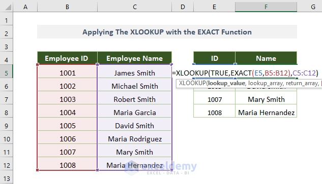
After entering the formula, the output looks as follows.

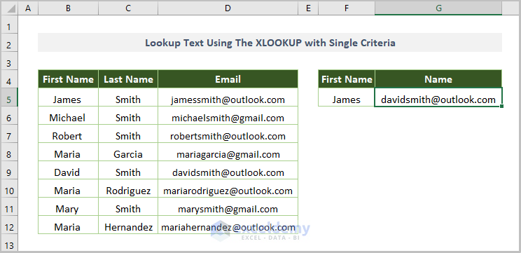
Method 6 – Using XLOOKUP with Single Criteria to Lookup Text
Assuming that the employee name is divided into separate columns (one is the first name and the other one is the last name).
We’ll find the email of the first name easily with the XLOOKUP function.
The adjusted formula is:
= XLOOKUP(F5,B5:B12, D5:D12, 0, -1 ) F5 is the lookup value, B5:B12 is the lookup array that contains the lookup value, C5:C12 is the return cell range as we want to find the name, 0 is for if the value is not found, and -1 refers to match mode.
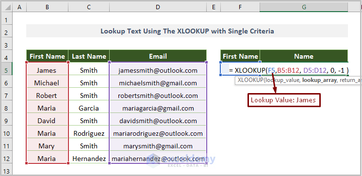
The output will be as follows.
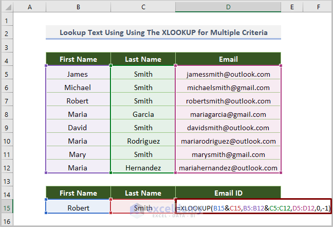
Method 7 – Utilizing XLOOKUP for Multiple Criteria to Lookup Text
We’ll extract the text value that matches multiple criteria using the flexible XLOOKUP function.
If you want to find the email based on the First Name and Last Name, use the following formula:
=XLOOKUP(B15&C15,B5:B12&C5:C12,D5:D12,0,-1)B15 is the first name, and C15 is the last name, B5:B12 is the lookup array (cell range for the First Name), C5:C12 is another lookup array (cell range for the Last Name), 0 is for if the value is not found, and -1 is the match mode.
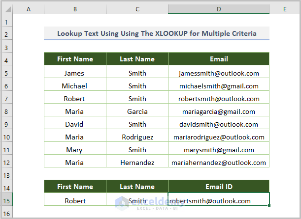
After inserting the above formula, you’ll get the output like the following picture.
Download the Practice Workbook
<< Go Back to Lookup | Formula List | Learn Excel
Get FREE Advanced Excel Exercises with Solutions!

Hi
Is possible to sum all WA11?
(A1) WA11 4
(A2) AdBlue 1, WA11 223
(A3) AdBlue 3, WA11 32, shift 4
… and everything is in one column.
Thanks you very much for your help.
Sincerely Marko
Hi Marko
I hope you are doing well.
After going through your problem, I will give you 2 possible solutions.
Solution 1:
This will require you to insert the number after “WA11” within parentheses.
● Add the parentheses.
● Then, write down the following formula in B2.
=MID(A1,SEARCH("(",A1)+1, SEARCH(")",A1)-SEARCH("(",A1)-1)+0● Then, press ENTER. Excel will extract the number inside the parentheses.
● Then, AutoFill up to B3.
● Finally, add the numbers.
Solution 2:
● This will require you to have a helping column with the numbers with “WA11”. But this is a bit tedious if you have a lot of data.
● Now, add the numbers.
Hope this helps. Thank you.