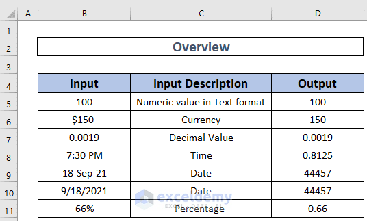
In this article we will demonstrate how to use Excel’s VALUE function to convert various types of data into numbers. Here is an overview:
Before diving into the examples, let’s introduce the VALUE function.
Summary:
Converts a text string that represents a number to a number.
Syntax:
VALUE(text)
Arguments:
text – The text value to convert into a number.
Version:
Available from Excel 2003.
Let’s put this function to work in some examples.
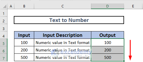
Example 1 – Converting Text Format to Number Format
Sometimes, whether by mistake or deliberately, a number can be formatted as a text value, meaning generic numeric operations can’t be performed on it. We can use the Value function to convert it to a number.
Steps:
- In cell D5, enter the following formula:
=VALUE(B5)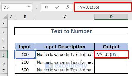
- Press ENTER to return the output.
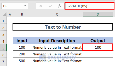
- Use the Fill Handle to AutoFill down to cell D7.
Example 2 – Converting Currency Format to Number Format
Steps:
- In cell D5, enter the following formula:
=VALUE(B5)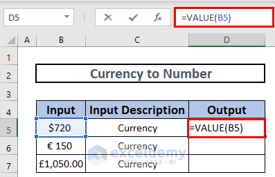
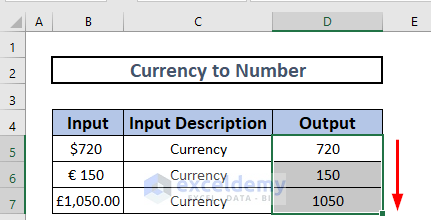
- Press ENTER to return the output.
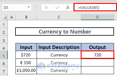
- Use the Fill Handle to AutoFill down to cell D7.
Example 3 – Converting Date-Time Format to Number Format
Steps:
- In cell D5, enter the following formula:
=VALUE(B5)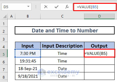
- Press ENTER to return the output.
- Use the Fill Handle to AutoFill down to cell D7.
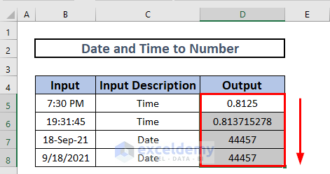
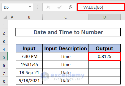
Note
Excel has inbuilt numeric values for times and date, so these numeric values will be returned when applying the VALUE function. For example, the numeric value for 7:30 PM is 0.8125.
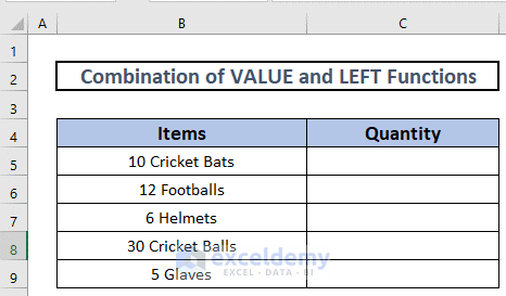
Example 4 – Combining the VALUE and LEFT Functions
In the case of data containing a combination of numbers and text strings, to retrieve the number and make sure that the value is in the number format we’ll use a helper function along with VALUE.
Here we have listed several items along with the quantity at the start of the string. We’ll extract the quantity value from these strings.
Steps:
Since the numeric values are on the left of the string, we will use the LEFT function, which retrieves a specific number of characters from the left of a string.
- Our formula in cell D5 is:
=VALUE(LEFT(B5,2))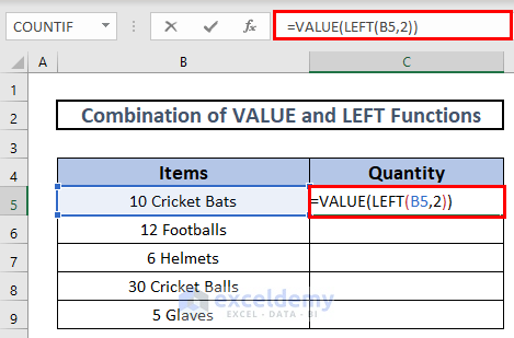
Formula Explanation
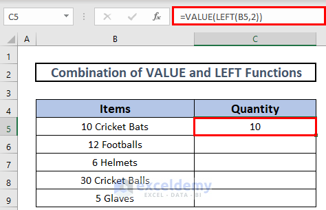
The LEFT function extracts the first 2 characters from the string, and then VALUE converts those characters into a number.
The desired result is returned.
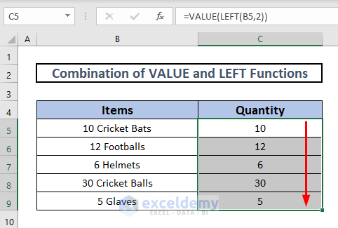
- Do the same for the rest of the values.
Example 5 – Merging the VALUE and IF Functions
Now we’ll demonstrate an advanced use of the VALUE function.
Suppose we have a dataset of a few employees with their entry and exit times. The duration of their work time is found by subtracting the entry time from the exit time.
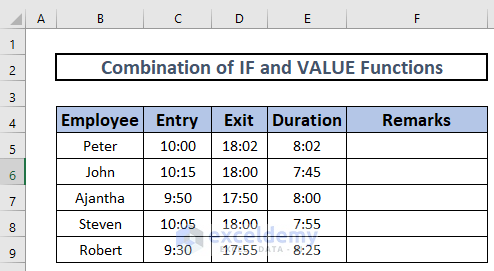
Suppose we want to check whether the employees are working the entire 8 hours, or less. We’ll use the IF function in combination with VALUE.
Steps:
- In cell D5, enter the following formula:
=IF(E5>=VALUE("8:00"),"Complete","Short")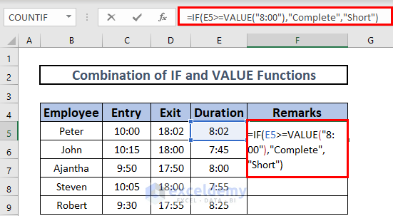
- Here we insert “8:00” within the VALUE function, convert the time to a number, then check if the duration value (E5) is greater than or equal to 8:00. If TRUE the formula will return “Complete”, otherwise “Short”.
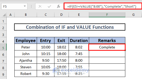
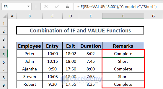
The duration is greater than 8 hours, so the output is “Complete”. When the duration is less than 8 hours, the output will be “Short”.
- Copy the formula to the rest of the cells.
Quick Notes
- Instead of cell references, we can directly insert values into the VALUE function.
- The VALUE function works perfectly with negative numeric values.
- A text string that cannot be converted to a number will return a #VALUE error.
- Inserting a text string without double quotes will return a #NAME? error.
Download Practice Workbook
<< Go Back to Excel Functions | Learn Excel
Get FREE Advanced Excel Exercises with Solutions!

I am multiplying my B column * my C column. But my C9 has an ‘-‘ entry.
I see that Value (C9) is going to give me an #VALUE error.
How can I use this?
Such as: =if(Value(C9) = “#VALUE”, 0, B9 * c9)
Hello John Wood,
You’re right, using VALUE(C9) when C9 contains a non-numeric value like “-” will result in a #VALUE! error.
To handle this, you can use the IFERROR function to avoid the error and replace it with 0 for the multiplication.
Formula:
=B9 * IFERROR(VALUE(C9), 0)
This way, if C9 contains something that can’t be converted to a number (like “-“), VALUE(C9) will throw an error, and IFERROR will catch it and return 0 instead preventing the #VALUE! error in your multiplication.
Regards
ExcelDemy