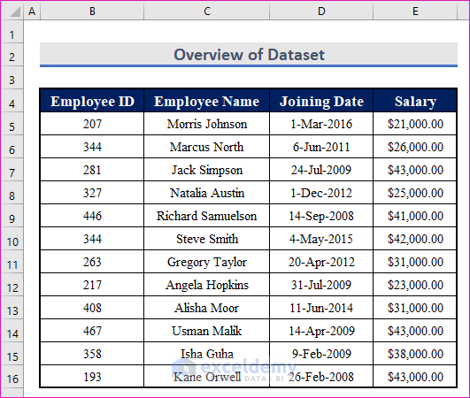
Consider the following dataset. We have the Employee IDs, Employee Names, Joining Dates, and Salaries of a company. We will lookup values with multiple criteria using the INDEX, MATCH, XLOOKUP, and FILTER functions.
Case 1 – Lookup with Multiple Criteria of AND Type in Excel
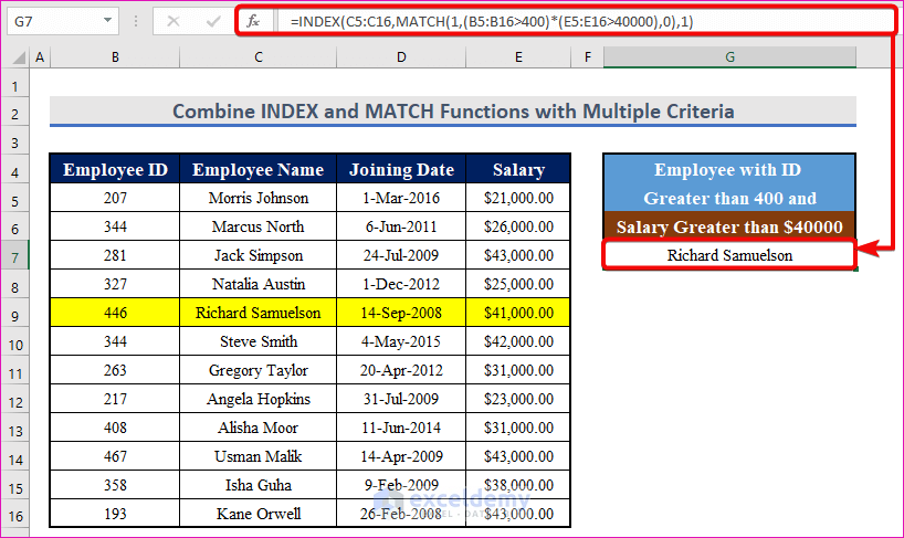
Let’s find an employee with an ID greater than 400 and a salary greater than $40,000.
Method 1.1 – Combining INDEX and MATCH Functions in Rows and Columns
Steps:
- Select cell G7 and insert the following formula.
=INDEX(C5:C16,MATCH(1,(B5:B16>400)*(E5:E16>40000),0),1)- Press Enter on your keyboard.
- B5:B16>400 goes through all the IDs in column B and returns an array of TRUE and FALSE, TRUE when an ID is greater than 400, otherwise FALSE.
- E5:E16>40000 goes through all the salaries in column E and returns an array of TRUE and FALSE, TRUE when a salary is greater than $40,000, otherwise FALSE.
- (B5:B16>400)*(E5:E16>40000) multiplies the two arrays of TRUE and FALSE, and returns a 1 when the ID is greater than 400 and the salary is greater than $40,000. Otherwise returns 0.
- MATCH(1,(B5:B16>400)*(E5:E16>40000),0) goes through the array (B5:B16>400)*(E5:E16>40000) and returns the serial number of the first 1 it encounters.
- In this case, it returns 5 because the first 1 is in serial number 5.
- INDEX(C5:C16,MATCH(1,(B5:B16>400)*(E5:E16>40000),0),1) returns the Employee name from the range C5:C16, with row number equal to the output of the MATCH function and column number equal to 1.
- Here’s the formula to find the employee who joined before 31 Dec, 2009, but still receives a salary lower than $25,000.
=INDEX(C5:C16,MATCH(1,(D5:D16<DATE(2009,12,31))*(E5:E16<25000),0),1)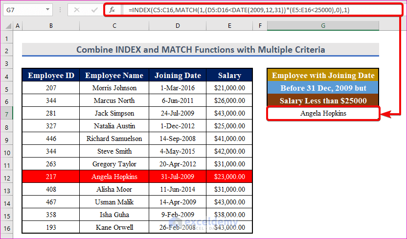
Method 1.2 – Using the XLOOKUP Function
XLOOKUP is only available in Excel 365.
Steps:
- Use the following formula in cell G7.
=XLOOKUP(1,(B5:B16>400)*(E5:E16>40000),C5:C16)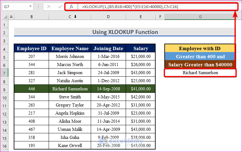
- (B5:B16>400)*(E5:E16>40000) returns an array of 1 and 0, 1 when the ID is greater than 400 and the salary is greater than $40,000. 0 otherwise.
- XLOOKUP(1,(B5:B16>400)*(E5:E16>40000),C5:C16) first searches for 1 in the array (B5:B16>400)*(E5:E16>40000). When it finds one, it returns the value from its adjacent cell in the range C5:C16.
Method 1.3 – Applying the FILTER Function
The INDEX-MATCH and the XLOOKUP formula have one limitation. If more than one value meets the given criteria, they return only the first value. To get all the values that satisfy the given criteria, you can use the FILTER function of Excel, but this one is also only available in Office 365.
Steps:
- Use the following formula in the result cell:
=FILTER(C5:C16,(B5:B16>400)*(E5:E16>40000))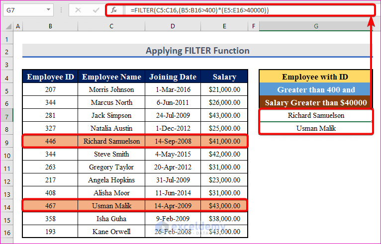
- (B5:B16>400)*(E5:E16>40000) returns an array of 1 and 0, 1 when the ID is greater than 400 and the salary is greater than $40,000. 0 otherwise (See the INDEX-MATCH section).
- FILTER(C5:C16,(B5:B16>400)*(E5:E16>40000)) goes through all the values in the array (B5:B16>400)*(E5:E16>40000), and when it finds a 1, it returns the adjacent value from the range C5:C16.
- Thus we get all the employees with an ID greater than 400 and a salary greater than $40,000.
- Here’s the formula to find the employees who joined between January 1, 2014, and December 31, 2016 and receive a salary of at least $30,000.
=FILTER(C5:C16,(D5:D16>=DATE(2014,1,1))*(D5:D16<=DATE(2016,12,31))*(E5:E16>=30000))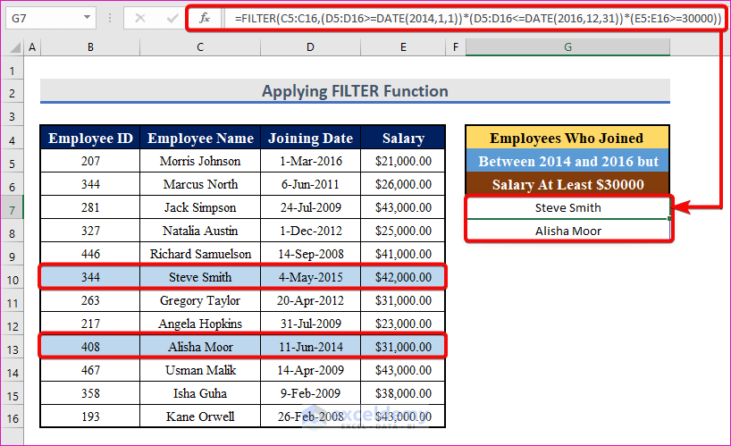
Case 2 – Lookup with Multiple Criteria of OR Type in Excel
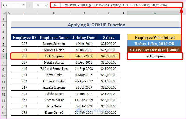
We’ll find an employee who joined before 1 Jan, 2010 or receives a salary greater than $30,000.
Method 2.1 – Merging INDEX and MATCH Functions in the Date Range
Steps:
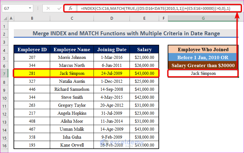
- Use the following formula:
=INDEX(C5:C16,MATCH(TRUE,((D5:D16<DATE(2010,1,1))+(E5:E16>30000))>0,0),1)Using INDEX-MATCH gets only the first value.
- D5:D16<DATE(2010,1,1) returns an array of TRUE and FALSE. TRUE when the joining date in column D is less than 1 Jan 2010. FALSE otherwise.
- E5:E16>30000 also returns an array of TRUE and FALSE. TRUE when the salary is greater than $30,000. FALSE otherwise.
- (D5:D16<DATE(2010,1,1))+(E5:E16>30000) adds the two arrays and returns another array of 0, 1, or 2. 0 when no criterion is satisfied, 1 when only one criterion is satisfied and 2 when both the criteria are satisfied.
- ((D5:D16<DATE(2010,1,1))+(E5:E16>30000))>0 goes through all the values of the array (D5:D16<DATE(2010,1,1))+(E5:E16>30000) and returns TRUE if the value is greater than 0 (1 and 2), and FALSE otherwise (0).
- MATCH(TRUE,((D5:D16<DATE(2010,1,1))+(E5:E16>30000))>0,0) goes through all the values in the array ((D5:D16<DATE(2010,1,1))+(E5:E16>30000))>0 and returns the first serial number where it gets a TRUE.
- In this case, returns 3 because the first TRUE is in serial 3.
- INDEX(C5:C16,MATCH(TRUE,((D5:D16<DATE(2010,1,1))+(E5:E16>30000))>0,0),1) returns the employee name from the range C5:C16 with the serial number returned by the MATCH function.
Here’s the formula to find the employee with an ID less than 300, or a joining date less than January 1, 2012, or a salary greater than $30,000:
=INDEX(C5:C16,MATCH(TRUE,((B5:B16<200)+(D5:D16<DATE(2012,1,1))+(E5:E16>30000))>0,0),1)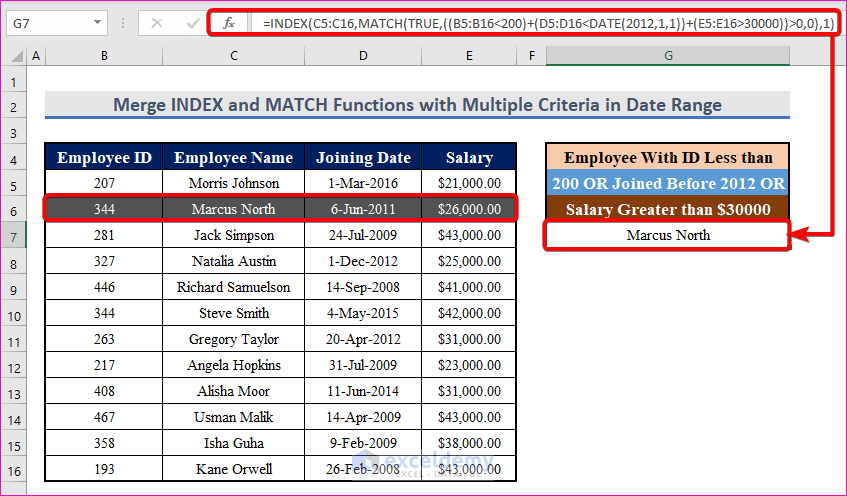
Method 2.2 – Applying the XLOOKUP Function
XLOOKUP is only available in Office 365.
Steps:
- The formula to find the employee with a joining date before January 1, 2010, or a salary greater than $30,000 will be:
=XLOOKUP(TRUE,((D5:D16<DATE(2010,1,1))+(E5:E16>30000))>0,C5:C16)This formula also returns the first value it finds.
- ((D5:D16<DATE(2010,1,1))+(E5:E16>30000))>0 returns TRUE when at least one of the two criteria is satisfied, otherwise FALSE. See the above section.
- XLOOKUP(TRUE,((D5:D16<DATE(2010,1,1))+(E5:E16>30000))>0,C5:C16) then returns the employee name from column C5:C16, where it gets the first TRUE.
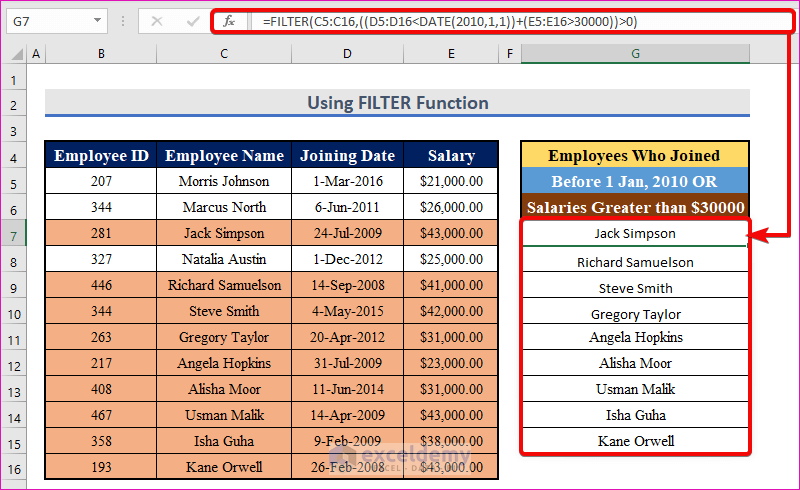
Method 2.3 – Using the FILTER Function
The FILTER function is only available in Office 365.
Steps:
- Use the following formula:
=FILTER(C5:C16,((D5:D16<DATE(2010,1,1))+(E5:E16>30000))>0)This formula returns all the employees who meet at least one of the given criteria.
- ((D5:D16<DATE(2010,1,1))+(E5:E16>30000))>0 returns TRUE when at least one of the two criteria is satisfied, otherwise FALSE. See the INDEX-MATCH section.
- FILTER(C5:C16,((D5:D16<DATE(2010,1,1))+(E5:E16>30000))>0) goes through all the cells in the range C5:C16 but returns only those when it encounters a TRUE.
Download the Practice Workbook
<< Go Back to Lookup | Formula List | Learn Excel
Get FREE Advanced Excel Exercises with Solutions!

Can I use lookup to populate the cells of one spreadsheet with the information from another using two separate criteria(date and text)? I’ve tried using Vlookup but I keep having issues with the date. Google sheets keep misinterpreting it.
Hi Temitope,
Our website currently focuses on providing articles and solutions for Microsoft Excel only. If you have the same problem in Excel, please provide us with a little bit more information. We will try to assist you as much as possible.