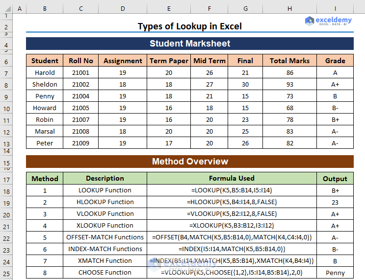
Here’s an overview of the functions and formulas for different types of lookups in Excel.
What Is a Lookup in Excel?
A lookup means searching for a specific value within a row or a column in Excel that meets specific criteria. You can look for single or multiple values within a range. There are several specific Excel built-in functions for looking up value both horizontally and vertically.
Different Types of Lookups to Apply in Excel: 8 Types
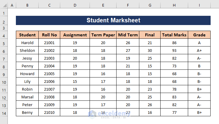
We have a list of marks obtained by different students throughout a semester in a subject. We will use it to demonstrate different lookup formulas.
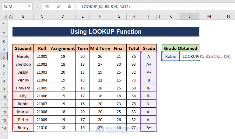
Method 1 – Using the LOOKUP Function in Excel
We want to find out the grade of one of the students, whose name is provided in the lookup cell K7.
Steps:
- Use the following formula,
=LOOKUP(K7,B5:B14,I5:I14)
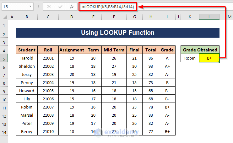
K7 is the lookup value, B5:B14 is the lookup array and I5:I14 is the result array. The LOOKUP function will find the lookup value in the lookup array and retrieve the corresponding value from the result array.
- Press Enter.
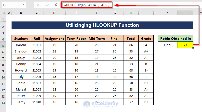
Method 2 – Utilizing the HLOOKUP Function for Horizontal Lookup
The HLOOKUP function looks for a value in the top row of a table or array and returns a value in the same column from a specified row. We want to find the mark obtained in the final by a student named Robin.
Steps:
- Apply the following formula.
=HLOOKUP(K5,B4:I14,8,FALSE)
Formula Breakdown
K5 is the lookup value, B4:I14 is the table array, 8 is the row index number which means we want the value from the 8th row of the table. FALSE indicates that the function will look for an exact match. The formula will search for the value of K5 (Final) in the top row of table B4:I14 and will return the value from the 8th row of the column in which K5 has been found.
Since the 8th row of the table array contains the scores for Robin, you will get the mark in the final obtained by Robin.
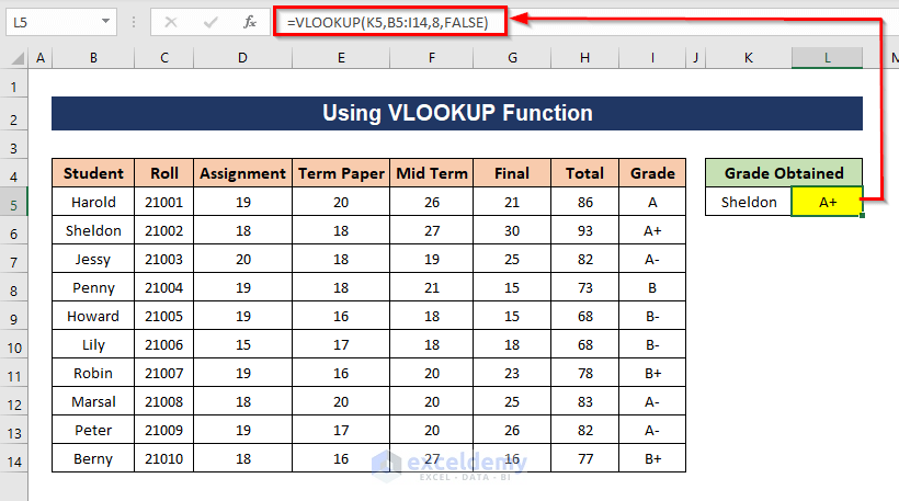
Method 3 – Lookup Vertically with the VLOOKUP Function
VLOOKUP looks for the value in the leftmost column and returns a value in the same row of the specified column. Let’s find out the grade of one of the students (Sheldon) using the VLOOKUP function.
Steps:
- Insert the following formula:
=VLOOKUP(K5,B5:I14,8,FALSE)
Formula Breakdown
K5 is the lookup value, B5:I14 is the table array, 8 is the column index number which means we want the value from the 8th column of the table array, and FALSE indicates that the function will search for an exact match. The function will look for K5 (Sheldon) in the leftmost column of table B5:I14 and will return the value of the 8th column from the row in which the lookup value has been found.
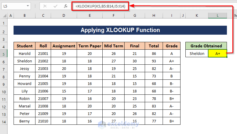
Method 4 – Applying the XLOOKUP Function for Excel 365
The XLOOKUP function searches a range or an array for a match and returns the corresponding item (position-wise) from a second range or array. It’s only available in Excel 365.
Steps:
- In cell L5, apply the following formula to get the grade of one of the students.
=XLOOKUP(K5,B5:B14,I5:I14)
Formula Breakdown
XLOOKUP searches for the value of K5 in the range B5:B14 and will return the corresponding value from the range I5:I14.
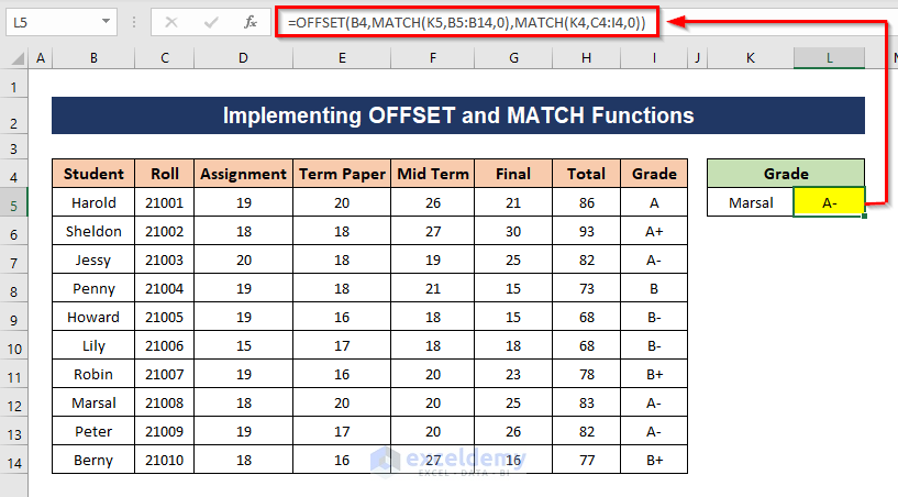
Method 5 – Implementing OFFSET and MATCH Functions
We will find out the grade of a student from the dataset.
Steps:
- Apply the following formula and press Enter to get the result.
=OFFSET(B4,MATCH(K5,B5:B14,0),MATCH(K4,C4:I4,0))
Formula Breakdown
B4 is the reference cell, which is the first cell of our dataset, K5 is the name of the student, B5:B14 is the range where the name of the student will be matched, K4 is the value that we are searching for (Grade), C4:I4 is the range from where the column of Grade will be matched. 0 is used to refer to an exact match. The formula will get the value from the intersecting cell of the Marsal (name of the student) row and the Grade column. It does that by offsetting the coordinates of the start of the table (B4) with the row value for Marsal and the column value for Grade, then returning the value in that cell.
Method 6 – Lookup a Value with INDEX and MATCH Functions
Steps:
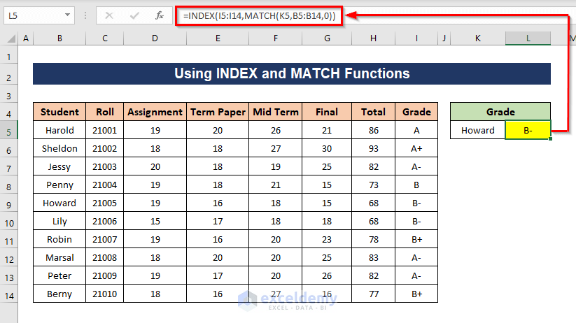
- Apply the following formula to find the grade of a student:
=INDEX(I5:I14,MATCH(K5,B5:B14,0))
Formula Breakdown
I5:I14 is the array from where the resulting value will be found, K5 is the lookup value, B5:B14 is the lookup array, and 0 indicates an Exact match. The MATCH function will return the position of the lookup value K5
MATCH(K5,B5:B14,0) => 5
The INDEX function will return the corresponding value from the I5:I14 array.
INDEX(I5:I14,MATCH(K5,B5:B14,0)) = =INDEX(I5:I14,5)
You will get the grade of the student in cell K5.
Method 7 – Employing the XMATCH Function to Lookup a Value
Steps:
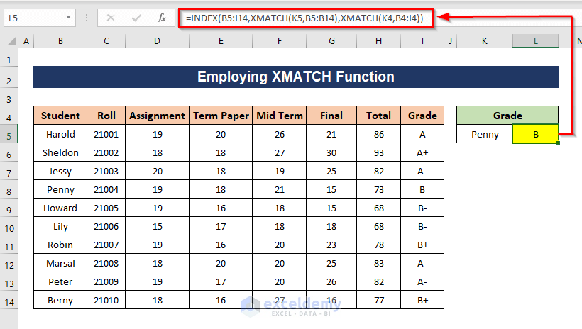
- Apply the following formula in a cell where you want to get the output:
=INDEX(B5:I14,XMATCH(K5,B5:B14),XMATCH(K4,B4:I4))
Formula Breakdown
The XMATCH functions will give the position of K5 from the range B5:B14 and the position of K4 from the range B4:I4.
XMATCH(K5,B5:B14) => 4 and XMATCH(K4,B4:I4) => 8
The INDEX function will use the position of K5 as the row number and the position of K4 as the column number in table B5:I14 to return the value of the cell at the intersection of that row and column.
INDEX(B5:I14,XMATCH(K5,B5:B14),XMATCH(K4,B4:I4)) = INDEX(B5:I14,4,8) = 8
You will get the grade of the student from cell K5.
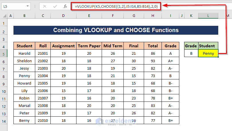
Method 8 – Combining VLOOKUP and CHOOSE Functions for Lookup in Excel
This formula will let us extract a value from the right to the left column.
Steps:
- Apply the following formula:
=VLOOKUP(K5,CHOOSE({1,2},I5:I14,B5:B14),2,0)
Formula Breakdown
The CHOOSE function will look for the corresponding data of column I in column B and return an array of these two data.
CHOOSE({1,2},I5:I14,B5:B14) => {“A”,”Harold”;”A+”,”Sheldon”;”A-“,”Jessy”;”B”,”Penny”;”B-“,”Howard”;”B-“,”Lily”;”B+”,”Robin”;”A-“,”Marsal”;”A-“,”Peter”;”B+”,”Berny”}
The VLOOKUP function will look for the cell value of K5 in that array and return the second value (column index 2) from that array which matches K5.
VLOOKUP(K5,CHOOSE({1,2},I5:I14,B5:B14),2,0) = VLOOKUP(K5,{“A”,”Harold”;”A+”,”Sheldon”;”A-“,”Jessy”;”B”,”Penny”;”B-“,”Howard”;”B-“,”Lily”;”B+”,”Robin”;”A-“,”Marsal”;”A-“,”Peter”;”B+”,”Berny”},2,0) = Penny
Download the Practice Workbook
<< Go Back to Lookup | Formula List | Learn Excel
Get FREE Advanced Excel Exercises with Solutions!

Download
Hello Aadirya Yadav
Thank you for your comment! You can download the related Excel file using the link below: Examples of Different Types of Lookups.xlsx
Keep exploring Excel with ExcelDemy!
Regards
ExcelDemy